pair source forward target reversed target
391 + 968 3 9 1 + 9 6 8 1 3 5 9 9 5 3 1
12 + 597 0 1 2 + 5 9 7 0 6 0 9 9 0 6 0
73 + 439 0 7 3 + 4 3 9 0 5 1 2 2 1 5 0
Homework 4: Attention and Transformers
Assignment Details
Assigned: 30 September
Due: Tuesday, 27 October at 23:59
Gradescope: Homework 4: Attention and Transformers | How to Submit
Starter: hw4-starter.zip
Requirements
- PyTorch >= 2.0
- Allowed libraries: PyTorch, NumPy, matplotlib, and the Python standard library
- No other external libraries unless a problem states an exception (no
nn.Transformer,nn.MultiheadAttention, pre-trained models, or attention libraries)
Overview
Three problems on attention: multi-head attention and an encoder-decoder for multi-digit addition, position encodings tested beyond the training length, and a decoder-only language model over molecule strings.
Getting Started
Download the starter code: hw4-starter.zip
unzip hw4-starter.zip
cd hw4-starter
python generate_datasets.py --seed 641
This creates datasets/addition (operand pairs for Problem 1),
datasets/offset (token sequences for Problem 2), and downloads
datasets/smiles (molecule strings for Problem 3). Use seed 641.
Each problem directory contains stub files with complete docstrings, a
test_interfaces.py suite, and a provided/ package. Run the tests
from inside each problem directory:
python -m pytest test_interfaces.py
The tests verify shapes, ranges, and conventions against hand-computed cases. They pass without any training and are part of the grading.
Data
The Datasets
generate_datasets.py generates the Problem 1 and 2 datasets with
seed 641 and downloads the Problem 3 dataset. This page renders the
Problem 1 and 2 examples from that script.
Addition
Operand pairs \((a, b)\) drawn uniformly from 0 to 999, deduplicated on
the unordered pair across splits: 10,000 training, 2,000 validation,
2,000 test pairs. The files hold only the pairs. The loader writes each
operand as three zero-padded digits and the sum as four, and reverses
the sum when digit_order is 'reversed'.
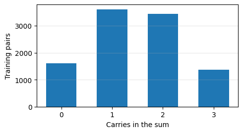
Carries per sum over the training split:
Offset Retrieval
Uniform random tokens from a vocabulary of 16: 20,000 training sequences of length 64 and 2,000 test sequences of length 128. The target at position \(i\) is the token at \(i - k\) with \(k = 7\). Positions \(0\) to \(6\) have no target.
position  0  1  2  3  4  5  6  7  8  9 10 11 12 13 14 15 16 17 18 19
token    11 15 11 11 11 14 10 14 10 12  8  9  6  3 13 13  4 11  2 10
target    .  .  .  .  .  .  . 11 15 11 11 11 14 10 14 10 12  8  9  6
Molecules
SMILES strings write a
molecule as a walk over its atoms: atom symbols
in order, = and # for double and triple bonds, parentheses for
branches, and a digit where a ring opens and the same digit where it
closes. Aromatic atoms are lower case. A bracket atom such as [nH]
carries explicit hydrogens.
CC(NC(=O)CSc1n[nH]c(N)n1)c1ccccc1Cl
Characters are the wrong unit: Cl is one atom, and [nH] is one
atom. The provided tokenizer splits the string into 31 tokens, and
joining the tokens reproduces the string.
C C ( N C ( = O ) C S c 1 n [nH] c ( N ) n 1 ) c 1 c c c c c 1 Cl
The dataset is a fixed subsample of the MOSES benchmark (drug-like
molecules from ZINC, MIT license): 100,000 training and 10,000
validation strings, 13 to 50 tokens each, mean 35. The vocabulary has
22 chemistry tokens: # ( ) - 1 2 3 4 5 = Br C Cl F N O S [nH] c n o s.
No charges, no stereochemistry, no ring digit above 5. Sixteen training
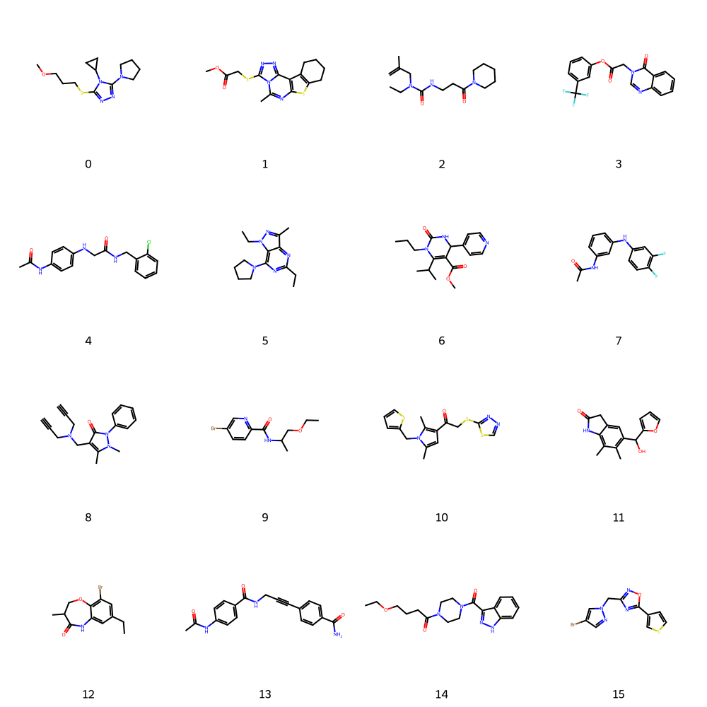
molecules, drawn with RDKit:
Problem 1
Problem 1: Transformer for Multi-Digit Addition
Requirements
Implement everything yourself except the files under provided/
(visualization). Do not modify provided files. No nn.Transformer,
nn.MultiheadAttention, or F.scaled_dot_product_attention in this
problem.
Build scaled dot-product attention, multi-head attention, and the encoder and decoder layers of a small transformer, then train it to add two three-digit numbers. The experiment is the order of the sum’s digits: most significant first, or least significant first. Train both orders on 1,000, 2,000, and 4,000 operand pairs with the same step budget, then read the attention maps and remove heads one at a time.
Part A: Dataset
Implement AdditionDataset in dataset.py:
- Constructor takes the data directory, the split name,
digit_order('forward'or'reversed'), andmax_pairs, which keeps the firstmax_pairspairs of the split - Items are
(src, tgt_in, tgt_out):srcis the 7-token sequencea2 a1 a0 + b2 b1 b0with zero-padded operands,tgt_outthe four zero-padded digits of the sum indigit_order, andtgt_intheBOStoken followed by the first three digits oftgt_out
Token ids are the digits 0 to 9, PLUS = 10, BOS = 11. The reversed
order reverses the sum only, never the operands.
Part B: Attention
Implement attention.py. Masks are boolean, True where attention is
allowed, and broadcast to \([B, h, T_q, T_k]\).
scaled_dot_product_attention(q, k, v, mask): \(\text{softmax}(q k^\top / \sqrt{d_k})\,v\) over \([B, h, T, d_k]\) tensors, masked positions removed before the softmax. Returns the output and the weights \([B, h, T_q, T_k]\).causal_mask(size, device): \([T, T]\), True on and below the diagonal.MultiHeadAttention(d_model, num_heads): projectionsW_q,W_k,W_v,W_o, eachnn.Linear(d_model, d_model). Head \(i\) reads columns \(i d_k\) to \((i+1) d_k\) of the projected queries, keys, and values, and its output entersW_othrough the same input columns. Returns the output \([B, T_q, d_{\text{model}}]\) and the weights.
Part C: Layers
Implement the forward passes of EncoderLayer and DecoderLayer in
model.py. The constructors are provided. Layers are post-norm, as in
Vaswani et al.:
| Layer | Sublayers |
|---|---|
| Encoder | \(x = \text{LN}(x + \text{Dropout}(\text{SelfAttn}(x)))\), then \(x = \text{LN}(x + \text{Dropout}(\text{FFN}(x)))\) |
| Decoder | masked self-attention, then cross-attention with queries from \(y\) and keys and values from the encoder output, then the FFN, each wrapped the same way |
FFN is Linear(\(d_{\text{model}} \to d_{\text{ff}}\)) \(\to\) ReLU \(\to\) Linear(\(d_{\text{ff}} \to d_{\text{model}}\)). Each layer returns its attention weights alongside its output.
The stack is provided: 2 encoder and 2 decoder layers,
\(d_{\text{model}} = 128\), \(h = 4\), \(d_{\text{ff}} = 256\), dropout 0.1,
one token embedding and one sinusoidal position table shared by source
and target, and greedy generate. The provided embedding uses
standard deviation \(d_{\text{model}}^{-1/2}\) at initialization and
multiplies by \(\sqrt{d_{\text{model}}}\) in the forward pass. With
PyTorch’s default initialization and the same multiply, the position
signal is a tenth of the token signal and the model does not learn the
task.
Part D: Training
Complete train.py. The configuration is fixed: Adam, learning rate
\(10^{-3}\), batch size 128, 2,400 steps, validation every 50 steps.
validate measures accuracy under greedy decoding, not teacher
forcing. Each run is named {digit_order}_n{train_size}.
python train.py --digit_order forward --train_size 1000
python train.py --digit_order forward --train_size 2000
python train.py --digit_order forward --train_size 4000
python train.py --digit_order reversed --train_size 1000
python train.py --digit_order reversed --train_size 2000
python train.py --digit_order reversed --train_size 4000
The log results/training_log_{run}.json records the step, the
training loss, validation exact match and token accuracy at every
evaluation, and steps_to_95, the first logged step at which
validation exact match reaches 0.95. train.py saves the final
weights to results/model_{run}.pth.
Part E: Analysis
Complete evaluate.py. For each run present it records test exact
match, test token accuracy, and steps_to_95 in
results/metrics.json, keyed by run name. On the two n4000 models:
remove_headzeroes one head’s input columns ofW_o;single_head_ablationreports test exact match with each of the 24 heads removed alone, undermetrics.json['ablation']greedy_pruningremoves heads one at a time, each time the head whose removal costs the least, with the cost recomputed after every removal, undermetrics.json['pruning']mean_attention_mapsaverages the encoder self-attention and decoder cross-attention weights over the test split, with the decoder fed its own greedy predictions
Visualizations, through provided/visualize.py: validation exact
match against step for the six runs on one figure, test exact match
against training size per order, the mean cross-attention maps per
decoder layer and head and the mean encoder self-attention maps per
layer and head for both n4000 models, and the pruning curves.
Deliverables
See Submission.
a. results/metrics.json and the six training logs.
b. The visualizations of Part E.
c. Report: test exact match and steps_to_95 for all six runs. The
effect of digit order at each training size, explained from what
output step \(j\) must know about the input in each order. The
cross-attention maps: which source positions each output step reads
in the last decoder layer, and where the network reads the carry
into place \(j\), argued from the layer-0 maps. The single-head
table and the pruning curve: how many heads the model needs, and
whether the heads that matter under single removal are the ones
that survive pruning.
Problem 2
Problem 2: Position Encodings and Length Extrapolation
Requirements
Implement everything yourself except the files under provided/ (the
one-layer attention model, visualization). Do not modify provided
files.
A provided one-layer, single-head causal attention model learns offset retrieval: at every position \(i \geq k\) the target is the token at position \(i - k\), with \(k = 7\). The tokens carry no information about position, so position information alone solves the task. Compare four ways of supplying it: none, a learned table, the sinusoidal table added to the embedding, and rotary encoding applied to queries and keys. Training sequences have 64 positions. Test sequences have 128, so positions 64 to 127 never occur in training.
Part A: Dataset
Implement OffsetDataset in dataset.py:
- Constructor takes the data directory, the split name, and \(k\)
- Items are
(tokens, targets): a[T]long tensor of tokens in \([0, 16)\) and a[T]long tensor withtokens[i - k]at every \(i \geq k\) andIGNORE_INDEX(\(-100\)) at \(i < k\)
Part B: Sinusoidal Table
Implement sinusoidal_table(max_len, d_model) in positional.py. Row
\(p\) holds, for \(i = 0, \dots, d_{\text{model}}/2 - 1\),
\[
\text{PE}[p, 2i] = \sin(p\,\theta_i) \qquad
\text{PE}[p, 2i+1] = \cos(p\,\theta_i) \qquad
\theta_i = 10000^{-2i / d_{\text{model}}}
\]
Implement shift_rotation(shift, d_model): the \(d_{\text{model}} \times
d_{\text{model}}\) matrix \(R_s\) with \(\text{PE}[p + s] = R_s\,\text{PE}[p]\)
for every \(p\). \(R_s\) is block diagonal with one \(2 \times 2\) block per
pair \((2i, 2i+1)\). Derive the block from the angle-addition identities.
evaluate.py measures the identity’s error over several \((p, s)\)
pairs.
Part C: Rotary Encoding
Implement rotary_frequencies(d_model) and apply_rotary(x, positions). Rotary encoding adds no vector. It rotates each pair
\((2i, 2i+1)\) of a query or key at position \(p\) by the angle
\(p\,\theta_i\), with the same \(\theta_i\) as above and the same
interleaved pair layout:
\[
\begin{bmatrix} x'_{2i} \\ x'_{2i+1} \end{bmatrix} =
\begin{bmatrix} \cos p\theta_i & -\sin p\theta_i \\
\sin p\theta_i & \cos p\theta_i \end{bmatrix}
\begin{bmatrix} x_{2i} \\ x_{2i+1} \end{bmatrix}
\]
Implement score_shift_invariance(q, k, shift, scheme): the absolute
change in the attention score \(q^\top k\) of one query and one key when
both positions move by shift. Scheme 'rotary' rotates both vectors
with apply_rotary. Scheme 'sinusoidal' adds the table row of each
position to each vector before the dot product. The rotary score
depends on the two positions only through their difference. The
function measures whether the same holds for the sinusoidal score.
Part D: Training
Complete train.py. The configuration is fixed: Adam, learning rate
\(10^{-3}\), batch size 64, 5 epochs, \(d_{\text{model}} = 64\), one head.
The model is provided. --position selects the scheme and names the
run.
python train.py --position none
python train.py --position learned
python train.py --position sinusoidal
python train.py --position rotary
The learned table has 128 rows. The embedding is not scaled by \(\sqrt{d_{\text{model}}}\): on unit-variance embeddings the scale would make the position signal an eighth of the token signal.
The log records per-epoch loss and accuracy over positions with a
target, on the training split and on the first 64 positions of the
test split, in results/training_log_{position}.json. Weights are
saved to results/model_{position}.pth.
Part E: Evaluation
Complete evaluate.py. For each run present it records in
results/metrics.json, keyed by position scheme, the accuracy over
positions 0 to 63 (in_range), over 64 to 127 (beyond), and over
the four 16-position buckets beyond (beyond_buckets). A top-level
checks entry records shift_rotation_max_error,
rotary_score_shift_error, sinusoidal_score_shift_error, and
rotary_vs_pairwise_error, the last against an explicit per-pair
rotation written in evaluate.py. Visualizations:
- Accuracy per 16-position bucket over 0 to 127 for the four schemes on one figure, with the training length marked
- Attention maps of one test sequence for the sinusoidal and rotary models, positions 0 to 31 and 96 to 127 side by side
Deliverables
See Submission.
a. results/metrics.json and the four training logs.
b. The visualizations of Part E.
c. Report: the in-range and beyond accuracies of the four schemes, with
the bucket curve. What the learned table does at positions 64 to
127, explained from which rows received gradient during training.
The two checks and what each one establishes about the sinusoidal
and rotary encodings, connected to the measured accuracies beyond
the training length. The attention maps in both windows, compared
between the two encodings.
Problem 3
Problem 3: Decoder-Only Transformer for SMILES
Requirements
Implement everything yourself except the files under provided/
(SMILES tokenizer, RDKit chemistry helpers, visualization). Do not
modify provided files. F.scaled_dot_product_attention is permitted
in this problem. RDKit is permitted through provided/chem.py only.
Compute
A GPU is recommended for this problem. Google Colab is sufficient for every run.
Build a GPT-style language model over SMILES strings and train it many times, briefly. The experiment is whether a run trains at all as a function of three choices: where the LayerNorm sits in each block, the learning rate, and warmup. The domain supplies a measure beyond loss: a sampled string either describes a molecule or it does not. You write the syntactic check, and RDKit decides the chemistry.
Part A: Dataset
Implement build_vocab and SmilesDataset in dataset.py:
build_vocabreturns the providedSmilesVocabover every token of the training file- Items are
(input_ids, target_ids), each[max_len - 1]long: encode the string as[BOS, tokens, EOS], pad withPADtomax_lenids, take every id but the last as the input and every id but the first as the target, withIGNORE_INDEX(\(-100\)) where the target isPAD
Part B: Model
Implement model.py. causal_mask(size, device) is boolean, True on
and below the diagonal.
Block(d_model, num_heads, d_ff, dropout, norm):
norm |
Block |
|---|---|
'post' |
\(x = \text{LN}(x + \text{Dropout}(\text{SelfAttn}(x)))\), then \(x = \text{LN}(x + \text{Dropout}(\text{FFN}(x)))\) |
'pre' |
\(x = x + \text{Dropout}(\text{SelfAttn}(\text{LN}(x)))\), then \(x = x + \text{Dropout}(\text{FFN}(\text{LN}(x)))\) |
Self-attention: q, k, v, and output projections
Linear(\(d_{\text{model}} \to d_{\text{model}}\)), \(h\) heads,
F.scaled_dot_product_attention with your causal mask as attn_mask.
FFN: Linear(\(d_{\text{model}} \to d_{\text{ff}}\)) \(\to\) GELU \(\to\)
Linear(\(d_{\text{ff}} \to d_{\text{model}}\)).
DecoderLM(vocab_size, d_model, num_layers, num_heads, d_ff, max_len, dropout, norm): token embedding plus a learned position embedding,
neither scaled, dropout, num_layers blocks, a final LayerNorm for
'pre' only, and a linear head to the vocabulary. Configuration:
\(d_{\text{model}} = 128\), \(h = 4\), \(d_{\text{ff}} = 512\), 4 layers,
dropout 0.1, max_len 52. PyTorch’s default initialization throughout.
Part C: Training
Complete train.py. Adam with betas \((0.9, 0.98)\), batch size 128,
gradient clipping at norm 1.0, 1,500 steps unless --steps says
otherwise. lr_at_step(step, peak_lr, warmup) rises linearly from 0 to
the peak over warmup steps and holds the peak after. The training
step records the gradient norm of the output head’s weight and the
total gradient norm before clipping. Measure validation loss every
250 steps and at the end. Each run is named
{norm}_lr{lr}_w{warmup}_s{steps}.
The sweep is twelve runs:
python train.py --norm {pre,post} --lr {1e-3,1e-2,3e-2} --warmup {0,500}
Then one longer run, with checkpoints for Part E:
python train.py --norm pre --lr 1e-3 --warmup 500 --steps 4000 --checkpoint_every 1000
The log results/training_log_{run}.json records the step, training
loss, learning rate, and the two gradient norms every 50 steps, the
validation losses, and the configuration. Save weights to
results/model_{run}.pth and checkpoints to
results/model_{run}_step{N}.pth.
Part D: Sampling and Well-Formedness
Implement generate in sample.py: batched autoregressive sampling
from BOS, the next id drawn from \(\text{softmax}(\text{logits} / T)\)
at the last position, each sequence finished at EOS, decoded with
the vocabulary.
python sample.py --run pre_lr0.001_w500_s4000
Implement is_well_formed(smiles) in evaluate.py: the tokens rejoin
to the string, parentheses balance and never go negative, each ring
digit’s next occurrence closes it and none remains open at the end,
and bracket atoms close. Implement max_open_ring_span(smiles): the
longest distance in tokens between a ring digit and its closing
partner. Operate on the provided tokenize output.
Part E: Evaluation
Complete evaluate.py. A run trains if its final validation loss is
below 2.0. For each of the twelve _s1500 logs,
metrics.json['sweep'] records the run, its three settings, the final
validation loss, the verdict, and the mean and maximum of the logged
head gradient norm over the first 100 steps (the log points at steps
50 and 100).
For 1,000 samples at \(T = 1\) from each checkpoint and from the final
model, record under metrics.json['main']['by_step'] the well-formed
fraction, RDKit validity, uniqueness, and novelty against the training
set. For the final model, record the three outcome fractions (valid,
well-formed but invalid, ill-formed) by string length and by maximum
open ring span under by_length and by_span, and validity,
uniqueness, and novelty at \(T \in \{0.7, 1.0, 1.3\}\) under
by_temperature.
Visualizations, through provided/visualize.py: the sweep grid with
the threshold, the validity curve over checkpoints, the two failure
breakdowns, the property distributions (QED, logP, molecular weight) of
valid samples against 1,000 training molecules, and a grid of 16 valid
samples drawn with RDKit.
Deliverables
See Submission.
a. results/metrics.json, the thirteen training logs, and the sample
file.
b. The visualizations of Part E.
c. Report: the sweep as a table of verdicts over learning rate, norm
placement, and warmup, and what the loss curves of the failing runs
look like. What the early head gradient norms separate and what they
do not. The largest learning rate at which each norm placement
trains, with and without warmup, and the mechanism that accounts
for the difference, argued from where the LayerNorm sits relative
to the residual path. The validity curve: how the well-formed and
RDKit-valid fractions move over training, and what separates a
well-formed string from a valid molecule, with examples from your
samples. The failure breakdowns by length and by ring span, and
what they say about what the model finds hard. The temperature
sweep as a trade between validity and novelty.
Submission Requirements
Your GitHub repository must follow this exact structure:
<repo>/
├── generate_datasets.py
├── q1/
│   ├── dataset.py
│   ├── attention.py
│   ├── model.py
│   ├── train.py
│   ├── evaluate.py
│   ├── test_interfaces.py
│   ├── provided/
│   └── results/
│       ├── training_log_*.json
│       ├── metrics.json
│       └── visualizations/
├── q2/
│   ├── dataset.py
│   ├── positional.py
│   ├── train.py
│   ├── evaluate.py
│   ├── test_interfaces.py
│   ├── provided/
│   └── results/
│       ├── training_log_*.json
│       ├── metrics.json
│       └── visualizations/
├── q3/
│   ├── dataset.py
│   ├── model.py
│   ├── train.py
│   ├── sample.py
│   ├── evaluate.py
│   ├── test_interfaces.py
│   ├── provided/
│   └── results/
│       ├── training_log_*.json
│       ├── samples_*.txt
│       ├── metrics.json
│       └── visualizations/
├── report/
│   └── report.pdf
└── README.md
Do not commit datasets/ or model weights. The starter’s
.gitignore excludes both. report/report.tex is an optional LaTeX
template for the report: one section per problem, deliverable items in
order, figures embedded.
The README.md in your repository root contains your full name and
student ID. See the
submission guide for its
full contents.
Testing Your Submission
Before submitting:
- Your repository structure must match the requirement exactly
python -m pytest test_interfaces.pymust pass in every problem directory- Each problem’s training commands and
python evaluate.pymust run without errors - All output files must be generated in the correct locations