Homework 3: Generative Adversarial Networks and Variational Autoencoders
Assignment Details
Assigned: 16 September
Due: Tuesday, 29 September at 23:59
Gradescope: Homework 3: Generative Adversarial Networks and Variational Autoencoders | How to Submit
Starter: hw3-starter.zip
Requirements
- PyTorch >= 2.0
- Allowed libraries: PyTorch, NumPy, Pillow (PIL), matplotlib, and the Python standard library
- No other external libraries unless a problem states an exception (no torchvision.models, pre-trained models, or GAN libraries)
Overview
Two generative models: a conditional GAN for letter images, and a hierarchical VAE for drum patterns.
Getting Started
Download the starter code: hw3-starter.zip
unzip hw3-starter.zip
cd hw3-starter
python generate_datasets.py --seed 641
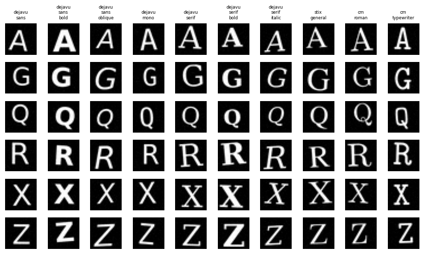
This creates datasets/fonts (28×28 grayscale letter images, A–Z in ten
typefaces) and datasets/drums (16×9 binary drum patterns in five
styles). Use seed 641.
Each problem directory contains stub files with complete docstrings, a
test_interfaces.py suite, and a provided/ package. Run the tests from
inside each problem directory:
python -m pytest test_interfaces.py
The tests verify shapes, ranges, and conventions against hand-computed cases. They pass without any training and are part of the grading.
Data
The Datasets
Both datasets are synthetic, generated by generate_datasets.py with seed
641. This page renders its figures from that generator.
Font Letters
28×28 grayscale images of the letters A–Z in ten typefaces, rendered from matplotlib’s bundled TTF files — the same files on every machine, so the dataset is identical everywhere. White glyph on black, per-sample affine jitter (shift, scale, rotation) and pixel noise. 200 training and 60 validation images per letter. Typefaces cycle within each letter, so font balance is exact. Images are stored as uint8 PNGs. The Problem 1 loader maps them to \([-1, 1]\).
One annotation record:
{
  "id": 0,
  "image_id": 0,
  "letter": "A",
  "letter_id": 0,
  "font_id": 0
}
Drum Patterns
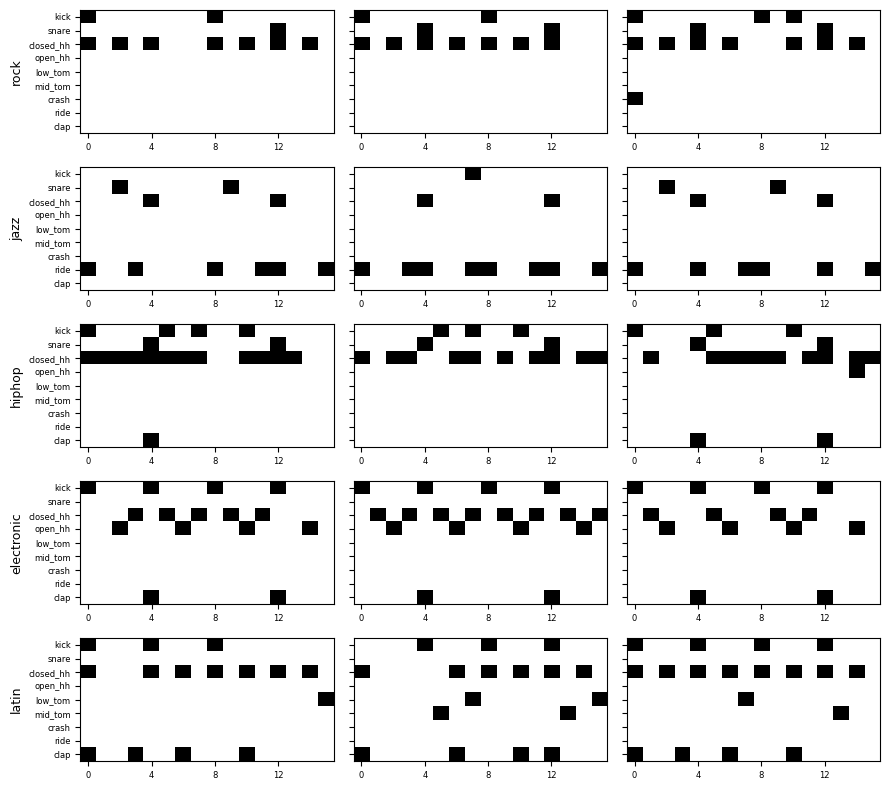
16×9 binary matrices: 16 timesteps (one bar of sixteenth notes) by 9 instruments — kick, snare, closed hi-hat, open hi-hat, low tom, mid tom, crash, ride, clap. Five styles (rock, jazz, hiphop, electronic, latin), 200 training and 60 validation patterns per style.
Style Templates
Each style is a matrix of per-cell hit probabilities. A pattern is one Bernoulli sample of its style’s matrix. The structure a model can learn is visible directly:
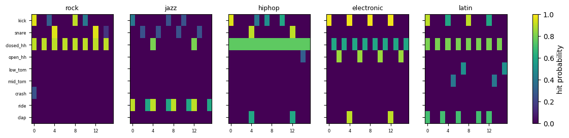
Pattern density differs by style — jazz is the sparsest, hiphop the densest. Problem 2’s latent analysis uses this.
Problem 1
Problem 1: Font Generation GAN
Requirements
Implement everything yourself except the files under provided/ (letter
classifier, coverage metrics, visualization). Do not modify provided
files.
Build a GAN that generates 28×28 letter images. The experiments: the two generator losses, unconditional training, and two conditional designs that differ only in where the discriminator sees the label. All are measured with the provided letter classifier.
Part A: Dataset
Implement FontDataset in dataset.py:
- Constructor takes the split’s image directory and annotation JSON
- Items are
(image, letter_id): a[1, 28, 28]float tensor in \([-1, 1]\) and a scalar long tensor in \([0, 26)\)
The \([-1, 1]\) range matches the generator’s Tanh output — the discriminator must see real and generated images on the same scale. The interface tests check it.
Part B: Models
Implement models.py. Both models take integer letter ids. Embeddings
live inside the models.
Generator(z_dim=100, num_classes=26, conditional=False):
| Stage | Layers |
|---|---|
| Unconditional projection | Linear(z_dim → 128·7·7) → BatchNorm1d → ReLU |
| Conditional projection | z: Linear(z_dim → 512); label: Embedding(26, 128); combined: Linear(640 → 128·7·7) → BatchNorm1d → ReLU |
| Upsampling (from [128, 7, 7]) | ConvTranspose2d(128 → 64, 4, stride 2, pad 1) → BN → ReLU, then ConvTranspose2d(64 → 1, 4, stride 2, pad 1) → Tanh |
Discriminator(num_classes=26, conditional=False, fusion='early'):
| Stage | Layers |
|---|---|
| features | Conv2d(in → 64, 4, stride 2, pad 1) → LeakyReLU(0.2), Conv2d(64 → 128, 4, stride 2, pad 1) → BN → LeakyReLU(0.2), Conv2d(128 → 256, 3, stride 2, pad 1) → BN → LeakyReLU(0.2) |
fusion='late' |
label: Embedding(26, 128), concatenated with the flattened features; classifier Linear(4096 + 128 → 1) |
fusion='early' |
label: Embedding(26, 28·28) reshaped to [1, 28, 28], concatenated with the image as a second input channel; classifier Linear(4096 → 1) |
The discriminator outputs a logit — no sigmoid in the model. Training
uses BCEWithLogitsLoss.
Part C: Vanilla Training
Complete train.py. The configuration is fixed: Adam, learning rate
2×10⁻⁴, betas (0.5, 0.999), batch size 64, 60 epochs.
The discriminator trains on real images (target 1) and generated images
(target 0, detached). The generator loss is non-saturating: minimize
\(-\log D(G(z))\). --g_loss saturating selects the saturating
alternative, minimize \(\log(1 - D(G(z)))\), the raw minimax objective.
The log records per-epoch means of d_loss, g_loss, and
g_grad_norm (the global L2 norm of the generator gradient after the
generator’s backward pass), and mode coverage every fifth epoch via the
provided mode_coverage over 1000 samples. The final-epoch generator is
saved to results/generator{suffix}.pth — use the .pth extension, so
the starter’s .gitignore keeps weights out of your repository.
python train.py
Part D: The Generator Loss
Two five-epoch probes, one per generator loss:
python train.py --g_loss saturating --epochs 5 --suffix _saturating
python train.py --g_loss nonsaturating --epochs 5 --suffix _nonsat_probe
evaluate.py plots the two g_grad_norm series on one figure.
Part E: Conditioning
Conditioning adds the letter label to both networks. The two runs differ only in where the discriminator sees it.
Train the late-fusion configuration first:
python train.py --conditional --fusion late --suffix _late_fusion
Evaluate its style-consistency grid (all 26 letters from one fixed z, several z) and its classifier agreement. Determine what this generator learned to do with z and with the label.
Then the early-fusion configuration:
python train.py --conditional --suffix _conditional
Compare the two on coverage, agreement, and the style grids.
Part F: Evaluation
Complete evaluate.py. For each of the three 60-epoch runs it records in
results/metrics.json — keyed vanilla, late_fusion, conditional —
the mode_coverage output, plus classifier agreement (overall and per
letter) for the two conditional runs, and writes to
results/visualizations/:
- Sample grids, letter histograms, coverage curves, and loss curves, one per run
- Latent interpolations (z interpolated between endpoint pairs, fixed label per row when conditional)
- Style-consistency grids for both conditional runs
- The Part D gradient-norm comparison
Deliverables
See Submission.
a. results/metrics.json and the five training logs.
b. The visualizations of Part F.
c. Report: what the loss curves and coverage show over the vanilla
run, and whether the loss values indicate when to stop training. The
gradient-norm comparison, explained with the gradient expressions
from lecture. What the late-fusion style grid shows the generator
does with z and with the label, explained from where the label
enters the discriminator. The early-fusion comparison. What letter
coverage does not measure, and which standard GAN evaluation metrics
share that limitation.
Problem 2
Problem 2: Hierarchical VAE for Drum Patterns
Requirements
Implement everything yourself except the files under provided/
(posterior-collapse diagnostics, visualization). Do not modify provided
files. sklearn.manifold.TSNE is permitted in evaluate.py only.
Build a two-level VAE with a learned conditional prior, train it with and without collapse treatment, and measure what each level of the hierarchy encodes.
Part A: Dataset
Implement DrumPatternDataset in dataset.py:
- Constructor takes the drum data directory and the split name
- Items are
(pattern, style): a[16, 9]float tensor with binary values and a scalar long tensor in \([0, 5)\)
Part B: Model
Implement HierarchicalDrumVAE(z_high_dim=4, z_low_dim=12) in
model.py. The generative model is
\[
p(z_{\text{high}}) = \mathcal{N}(0, I) \qquad
p(z_{\text{low}} \mid z_{\text{high}}) =
\mathcal{N}\!\left(\mu_p(z_{\text{high}}),\,
\sigma_p^2(z_{\text{high}})\right) \qquad
p(x \mid z_{\text{low}}, z_{\text{high}}) = \text{Bernoulli(logits)}
\]
where \(\mu_p, \sigma_p^2\) come from the prior network. Inference is a ladder: \(q(z_{\text{low}} \mid x)\) from the pattern encoder, then \(q(z_{\text{high}} \mid z_{\text{low}})\) from the sampled \(z_{\text{low}}\).
| Component | Layers |
|---|---|
| encoder_low (input transposed to [9, 16]) | Conv1d(9 → 32, 3, pad 1) → ReLU, Conv1d(32 → 64, 3, stride 2, pad 1) → ReLU, Conv1d(64 → 128, 3, stride 2, pad 1) → ReLU, Flatten → 512; Linear heads to \(\mu_{\text{low}}, \log\sigma^2_{\text{low}}\) |
| encoder_high | Linear(12 → 64) → ReLU → Linear(64 → 32) → ReLU; Linear heads to \(\mu_{\text{high}}, \log\sigma^2_{\text{high}}\) |
| prior_net | Linear(4 → 64) → ReLU → Linear(64 → 24), split into \((\mu_p, \log\sigma_p^2)\) |
| decoder (from \([z_{\text{high}}, z_{\text{low}}]\)) | Linear(16 → 512) → ReLU → Unflatten [128, 4], ConvTranspose1d(128 → 64, 3, stride 2, pad 1, out pad 1) → ReLU, ConvTranspose1d(64 → 32, 3, stride 2, pad 1, out pad 1) → ReLU, Conv1d(32 → 9, 3, pad 1), transposed to [16, 9] logits |
Interfaces (signatures and return shapes are in the stubs and tested):
reparameterize, encode, prior, decode(z_high, z_low=None, temperature=1.0) — z_low=None samples from the conditional prior, and
temperature divides the logits at generation time only — and forward,
which returns the reconstruction logits, both posteriors’ parameters, and
the conditional prior’s parameters at the sampled \(z_{\text{high}}\).
Part C: ELBO
Implement elbo_loss in train.py:
\[
\mathcal{L} = \text{BCE}(x, \text{logits})
+ \beta \, KL\!\left(q(z_{\text{low}} \mid x) \,\|\,
p(z_{\text{low}} \mid z_{\text{high}})\right)
+ \beta \, KL\!\left(q(z_{\text{high}} \mid z_{\text{low}}) \,\|\,
\mathcal{N}(0, I)\right)
\]
Both KL terms are between diagonal Gaussians. Per dimension,
\[
KL_d = \tfrac{1}{2}\left(\log\tfrac{\sigma_p^2}{\sigma_q^2}
+ \tfrac{\sigma_q^2 + (\mu_q - \mu_p)^2}{\sigma_p^2} - 1\right)
\]
Clamp each dimension at the free-bits floor (0.1 nats, provided
apply_free_bits) before summing. Reduction: BCE summed over the 16×9
pattern, KL summed over dimensions, both averaged over the batch.
Part D: Training
Complete train.py. The configuration is fixed: Adam, learning rate
10⁻³, batch size 32, 100 epochs.
kl_beta implements cyclical annealing: the run splits into 4 equal
cycles, and within each cycle \(\beta\) ramps linearly from 0 to 1 over
the first half and holds 1 over the second. Validation always scores the
plain ELBO (\(\beta = 1\), no free bits). Select the best model on it
and save it to results/best_model{suffix}.pth (use .pth so the
starter’s .gitignore keeps weights out of your repository). The log
records the loss components, \(\beta\), and the active dimension counts at
both levels on the validation split (provided
analyze_posterior_collapse) every epoch.
Run both configurations: the treated one, and the plain ELBO with both treatments off.
python train.py
python train.py --no_anneal --free_bits 0 --suffix _no_anneal
Part E: Analysis
Complete evaluate.py. For both runs it records in
results/metrics.json — keyed annealed, no_anneal — the saved best
model’s active-dimension counts and per-dim KLs, the val plain ELBO,
nearest-centroid style accuracy in \(\mu_{\text{high}}\) (centroids from
train, accuracy on val), and the correlation of each \(z_{\text{low}}\)
dimension with pattern density on val. Visualizations:
- The active-dimensions-over-training comparison of the two runs
- Training curves per run
- t-SNE of \(\mu_{\text{high}}\) colored by style, per run
- Hierarchy sampling: rows share one \(z_{\text{high}}\), columns draw \(z_{\text{low}}\) from the conditional prior
- Style swap: pairs of validation patterns decoded with exchanged \(z_{\text{high}}\)
Deliverables
See Submission.
a. results/metrics.json and both training logs.
b. The visualizations of Part E.
c. Report: the active-units curves and per-dim KLs of the two runs.
Compare the two runs’ plain ELBO and active-dimension counts, and
explain how the ELBO relates to the number of latent dimensions in
use. What the annealing schedule changes about the optimization. What
\(z_{\text{high}}\) and \(z_{\text{low}}\) each encode, argued from the
swap grid, the t-SNE, and the density correlations. How many
\(z_{\text{high}}\) dimensions carry KL, and what that says about the
style variable in this data.
Submission Requirements
Your GitHub repository must follow this exact structure:
<repo>/
├── generate_datasets.py
├── q1/
│   ├── dataset.py
│   ├── models.py
│   ├── train.py
│   ├── evaluate.py
│   ├── test_interfaces.py
│   ├── provided/
│   └── results/
│       ├── training_log.json
│       ├── training_log_saturating.json
│       ├── training_log_nonsat_probe.json
│       ├── training_log_late_fusion.json
│       ├── training_log_conditional.json
│       ├── metrics.json
│       └── visualizations/
├── q2/
│   ├── dataset.py
│   ├── model.py
│   ├── train.py
│   ├── evaluate.py
│   ├── test_interfaces.py
│   ├── provided/
│   └── results/
│       ├── training_log.json
│       ├── training_log_no_anneal.json
│       ├── metrics.json
│       └── visualizations/
├── report/
│   └── report.pdf
└── README.md
Do not commit datasets/ or model weights — the starter’s
.gitignore excludes both. report/report.tex is an optional LaTeX
template for the report: one section per problem, deliverable items in
order, figures embedded.
The README.md in your repository root contains your full name and
student ID. See the
submission guide for its
full contents.
Testing Your Submission
Before submitting:
- Your repository structure must match the requirement exactly
python -m pytest test_interfaces.pymust pass in both problem directoriespython train.pyandpython evaluate.pymust run without errors in each problem directory- All output files must be generated in the correct locations