Fixed Summary Gives Every Output the Same View of the Input
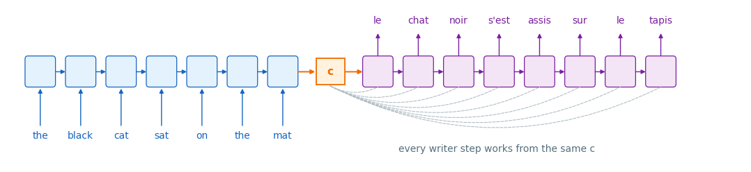
Encoder-decoder with one summary
- A reader runs over the source and keeps only its last state, \(\mathbf{c} = \mathbf{h}^{\text{enc}}_S \in \mathbb{R}^H\)
- A writer starts from \(\mathbf{c}\) and produces the target one word at a time
- \(\mathbf{c}\) is the only route from the source to every target word
Demands on one vector
- Carry every source word, and their order, in \(H\) numbers, for a source of any length
- Supply “black” when the writer reaches “noir” and “mat” when it reaches “tapis”, from the same vector
Measured on a reverse-copy task, \(S = 24\)
- Summary of \(H = 64\): the last three source words reproduced at 0.92 to 0.98, every earlier word at about 0.85
- \(H = 256\) reproduces every word at 0.99, with twelve times the recurrent parameters of \(H = 64\)
- The width needed grows with the source length, and every step of the reader and writer pays \(O(H^2)\) for it
Information already computed
- The reader computed one state per source word, \(\mathbf{h}^{\text{enc}}_1, \ldots, \mathbf{h}^{\text{enc}}_S\), and passed on only the last
Each Output Draws on Different Input Positions
Per target word
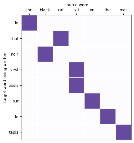
- “chat” corresponds to “cat”, “noir” to “black”, one position earlier in the source
- “s’est” and “assis” both correspond to “sat”
- A different source position, or a different pair, at almost every step
Fixed summary against this grid
- One vector serves all eight rows: each row must recover its own source word from the same encoding
- The reader’s per-position states are each closest to one source word, and none of them reaches the writer
Requirement from each row
- At each output, a vector built mostly from the input positions that output corresponds to
Weighted Read Gives Each Output Its Own Summary
One summary per output
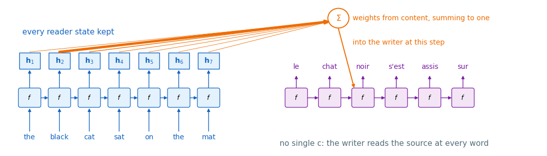
\[\mathbf{c}_t = \sum_{s=1}^{S} a_{t,s}\,\mathbf{h}^{\text{enc}}_s, \qquad a_{t,s} \ge 0, \quad \sum_s a_{t,s} = 1\]
- Every reader state is kept
- At each output \(t\), one weight per input position, computed from the writer’s state and that reader state
- \(\mathbf{c}_t\) changes from output to output: a soft version of the row of the grid
Measured on the same reverse-copy task
- With \(H = 64\) and the weighted read, every source word is reproduced at 0.998 or better, with 16% more parameters than the fixed-summary model
- The learned weights put most of each row on one reader state, the one that matches the word being written, with no alignment supplied
Open definitions
- How the weights are computed from the states: what similarity, how normalized, how sharp
- What a weighted average of stored vectors is, as an estimator, before any network is involved
Regression from Samples Averages the Outputs of Nearby Inputs
Setup
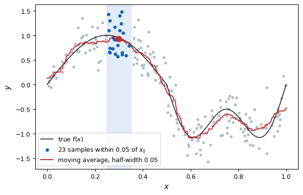
- \(n\) samples \((x_i, y_i)\) with \(y_i = f(x_i) + \varepsilon_i\), noise of variance \(\sigma^2\)
- Goal: the value \(f(x_0)\) at a query \(x_0\) that is not among the samples
Local averaging
- Inputs close to \(x_0\) have outputs close to \(f(x_0)\) when \(f\) is smooth
- Average the outputs \(y_i\) of the samples whose inputs \(x_i\) lie near \(x_0\)
- The estimate is a weighted sum of stored outputs, with weight \(1/m\) on the \(m\) samples inside the window and \(0\) elsewhere
Window
- Which samples count as near, and so how many are averaged
- No parameters are fitted: the samples are stored, and every query is answered from them
Kernel Weights Fall Off with Distance and Sum to One
Nadaraya-Watson estimator
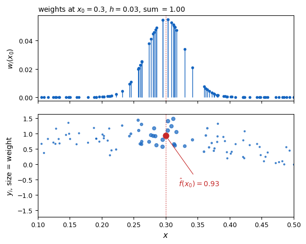
\[\hat f(x_0) = \sum_{i=1}^{n} w_i(x_0)\, y_i, \qquad w_i(x_0) = \frac{K\!\left(\frac{x_0 - x_i}{h}\right)}{\sum_{j} K\!\left(\frac{x_0 - x_j}{h}\right)}\]
- \(K\): a kernel, a bump centred at zero. Gaussian: \(K(u) = e^{-u^2/2}\)
- \(h\): the bandwidth. A sample at distance \(h\) from the query gets \(e^{-1/2} \approx 0.61\) of the weight of a sample at the query itself
- The box window is the kernel \(K(u) = [\,|u| \le 1\,]\)
Three properties of the weights
- Non-negative and summing to one: the estimate is an average of the stored outputs
- Set by the distance from the query to each stored input, not by the outputs
- Recomputed for every query: each \(x_0\) gets its own average
Bandwidth Sets How Many Samples Each Estimate Averages
Effective number of samples
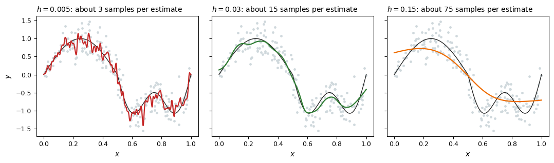
- The Gaussian weights reach about \(\sqrt{2\pi}\,h\) of input range around the query
- With \(n\) samples spread at density \(p(x)\), an estimate averages roughly \(m \approx n\,p(x_0)\,\sqrt{2\pi}\,h\) of them
- \(h = 0.005\): about 3 samples. \(h = 0.03\): about 15. \(h = 0.15\): about 75
Two ways to be wrong
- Few samples: each estimate is the average of a handful of noisy outputs, and it moves with their noise
- Many samples: the average reaches inputs where \(f\) has a different value, and the estimate is pulled away from \(f(x_0)\)
- The left panel shows the first, the right panel the second, and both at once on the wiggly half
Bandwidth Trades Variance Against Bias
Variance: averaging \(m\) noisy samples
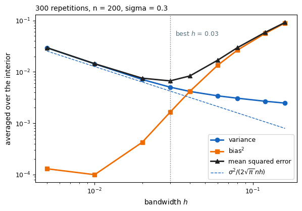
\[\mathrm{Var}\big[\hat f(x_0)\big] \approx \frac{\sigma^2}{n\,h\,p(x_0)}\cdot\frac{1}{2\sqrt{\pi}}\]
- The average of \(m\) independent outputs of variance \(\sigma^2\) has variance \(\sigma^2 / m\): its spread falls as \(1/\sqrt{m}\), not \(1/m\)
- With \(m \propto n h\), halving \(h\) doubles the variance
Bias: averaging a curved function
\[\mathbb{E}\big[\hat f(x_0)\big] - f(x_0) \approx \frac{h^2}{2}\, f''(x_0) \quad\text{(uniform } p\text{)}\]
- Inside the window \(f\) is approximately a parabola. The average of a parabola over a window centred at \(x_0\) differs from its centre value by the curvature times the window’s spread squared
- Where \(f\) curves fast, a wide window misses most. Where \(f\) is straight, any window is unbiased
Best bandwidth
- Minimizing the sum gives \(h^\star \propto n^{-1/5}\): more data allows a narrower window, slowly
- The best \(h\) depends on \(f''\) and \(p\), which differ from place to place
Gaussian Kernel Weights Are a Softmax over Scores
Expand the exponent
\[K\!\left(\tfrac{x_0 - x_i}{h}\right) = \exp\!\left(-\frac{x_0^2}{2h^2}\right)\exp\!\left(\frac{x_0\, x_i}{h^2}\right)\exp\!\left(-\frac{x_i^2}{2h^2}\right)\]
- The first factor is the same for every \(i\) and cancels in the normalization
\[w_i(x_0) = \frac{\exp\!\big(e_i / h^2\big)}{\sum_j \exp\!\big(e_j / h^2\big)}, \qquad e_i = x_0\, x_i - \tfrac{1}{2} x_i^2\]
- The weights are a softmax over the stored inputs of a score \(e_i\) divided by \(h^2\)
- In vectors, \(e_i = \mathbf{x}_0^\top \mathbf{x}_i - \tfrac12\|\mathbf{x}_i\|^2\): a dot product between query and stored input, plus a term in the stored input alone
Equal-norm stored inputs
- If every \(\|\mathbf{x}_i\|\) is the same, the second term cancels too, and the score is the dot product \(\mathbf{x}_0^\top \mathbf{x}_i\)
Bandwidth as temperature
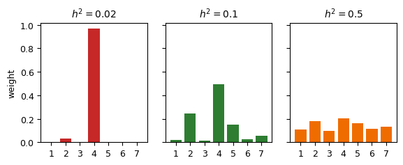
- \(h^2\) divides every score before the softmax: it is the softmax temperature
- \(h \to 0\): all weight on the highest score, the nearest sample alone, a hard lookup
- \(h \to \infty\): equal weights, the mean of all outputs
Fixed Kernel Applies One Notion of Closeness Everywhere
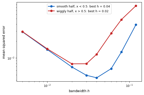
One bandwidth, two regions
- Measured: the smooth half’s error is smallest at \(h = 0.04\), the wiggly half’s at \(h = 0.02\)
- The smooth half is served by a wide window that averages away noise, the wiggly half by a narrow one that follows the function
- A single \(h\) is a compromise that is wrong on at least one side
One distance, every direction
- The kernel compares raw inputs by Euclidean distance: every coordinate counts, and counts equally
- With many input dimensions, most irrelevant to the output, the irrelevant ones dominate the distance and the nearest samples are not the relevant ones
- The kernel cannot learn which directions matter: it has no parameters
Requirement
- A similarity learned from the data, with its own directions and its sharpness set from the query