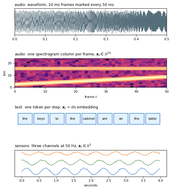
Sequences Are Lists of Vectors Indexed by Time
One vector per step
- \(\mathbf{x}_t \in \mathbb{R}^d\) at step \(t\), for \(t = 1, \ldots, T\)
- \(d\) set by the source, \(T\) by the example
Sources
| Source | Element \(\mathbf{x}_t\) | \(d\) | Rate |
|---|---|---|---|
| Text | one token, as an embedding vector | 100-1000 | one per word or subword |
| Audio | one frame of a mel spectrogram | 40-80 | 100 per second |
| Sensors | one reading of every channel | 3-50 | 50-1000 per second |
- Video: one frame’s feature vector, 25-30 per second
Examples Have Different Lengths
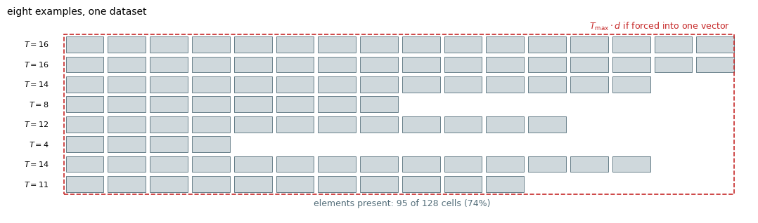
Lengths in three kinds of data
- Sentences in one corpus: 3 to 60 tokens
- Spoken utterances: 1 to 35 seconds, 100 to 3500 frames
- Recordings and logs: minutes to hours, \(T\) in the millions
Requirements on the model
- The input dimension \(T \cdot d\) differs from example to example
- A batch of examples is ragged: every row a different length
- Test examples can be longer than any training example
Element Order Matters
Examples
- “dog bites man” and “man bites dog” use the same three tokens
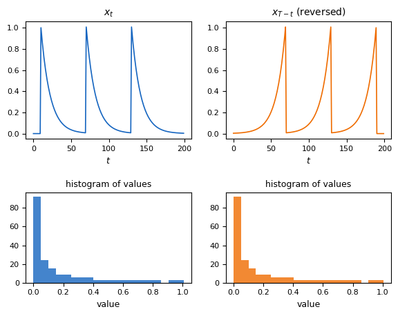
- A waveform and its time reversal have the same sample values and are different sounds
- A rising ramp and a falling ramp have the same set of values
Relative position
- The position of each element relative to the others
- Not its absolute position: “man bites dog” means the same at the start of a paragraph and at the end
Test
- Shuffle the elements of an input. An unchanged output means the order was never used
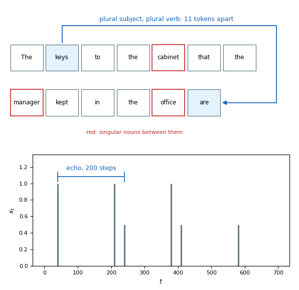
Dependent Elements Can Be Far Apart
Language
- “The keys to the cabinet that the manager kept in the office are on the table”
- The verb agrees with “keys”, eleven tokens back
- Three singular nouns in between, each of which the verb could wrongly agree with
Signals
- An echo: \(x_t\) reappears at \(t + 200\), attenuated
- A control input at \(t\) shows in the output only after the plant’s delay
- A fault at \(t\) changes statistics for the rest of the log
Required of a model
- Retention: information from step \(t - k\) must still be available at step \(t\), with \(k\) set by the data
- Selectivity: what arrives in between must not overwrite it
Feedforward Networks Need Each Sequence as \(D\) Numbers
First layer
- \(\mathbf{W}^{(1)} \in \mathbb{R}^{H \times D}\), with \(D\) chosen before any data is seen
- Every example must be a vector of exactly \(D\) numbers
Reshaping a sequence into \(D\) numbers
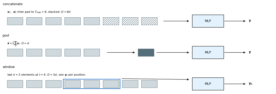
- Concatenate: pad or cut to \(T_{\max}\), stack the elements, \(D = T_{\max} \cdot d\)
- Pool: sum or average the elements, \(D = d\)
- Window: the last \(k\) elements at each step, \(D = k \cdot d\), one output per step
- Each keeps the network as it is and discards something: length beyond \(T_{\max}\), the order, or the elements outside the window
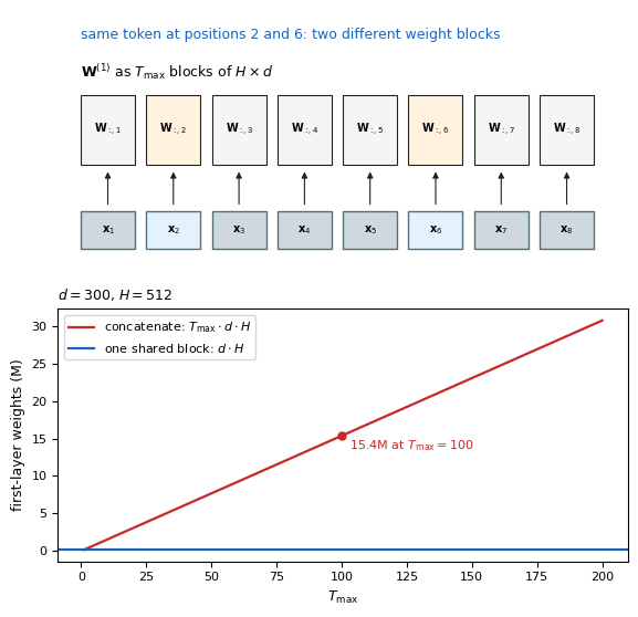
Concatenation Gives Every Position Its Own Weights
Parameter count
- \(\mathbf{W}^{(1)} \in \mathbb{R}^{H \times T_{\max} d}\)
- \(T_{\max} = 100\), \(d = 300\), \(H = 512\): \(15.4\)M weights in the first layer
- One \(H \times d\) block, shared across positions: \(154\)K
Separate weights per position
- Column block \(t\) of \(\mathbf{W}^{(1)}\) multiplies \(\mathbf{x}_t\) and nothing else
- A pattern learned at position 3 is unknown at position 40 until training shows it there
- Every pattern must appear at every position in the training data: data needed grows with \(T_{\max}\)
Length fixed at \(T_{\max}\)
- A longer example is cut
- A shorter example carries \(T_{\max} - T\) pad vectors, each still multiplied by its block
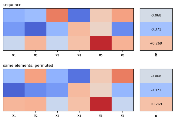
Pooling Discards Order
Sum or mean over \(t\)
- \(\bar{\mathbf{x}} = \frac{1}{T}\sum_{t=1}^T \mathbf{x}_t\), then a feedforward network on \(\bar{\mathbf{x}}\)
- Any \(T\), \(H \cdot d\) weights, shared across positions by construction
Permutation invariant, by construction
- Every ordering of the same elements gives the same \(\bar{\mathbf{x}}\)
- “dog bites man” and “man bites dog” are one input
Task dependence
- Enough: topic of a document, presence of a keyword, average loudness of a clip
- Not enough: agreement, translation, an echo, anything where relative position matters
Convolution Extends from Images to Sequences
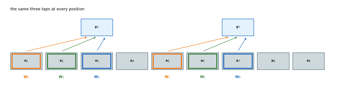
Across an image
- An image has no fixed size either: one \(k \times k\) kernel slides over every position
- Parameters depend on \(k\) and the channels, not on the image
Along time
\[\mathbf{y}_t = \sum_{j=0}^{k-1} \mathbf{W}_j\, \mathbf{x}_{t-j}\]
- A 1-D convolution: \(k\) taps, each an \(C \times d\) matrix
- \(k \cdot d \cdot C\) parameters for any \(T\)
- The same pattern detected at every position with the same weights
- An FIR filter with matrix taps
Properties
- Any \(T\), one output per step, every step computed in parallel
- Each output depends on exactly \(k\) steps, by construction
Receptive Field Is Fixed by Kernel Width and Depth
Receptive field
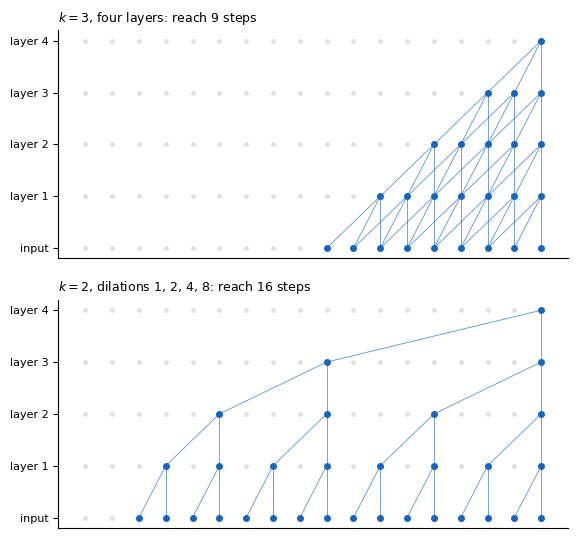
- One layer, \(k\) taps: an output covers \(k\) steps
- \(L\) layers, stride 1: \(1 + L(k - 1)\) steps. \(k = 3\), \(L = 10\): 21 steps
- Dilations \(1, 2, 4, \ldots, 2^{L-1}\) with \(k = 2\): \(2^L\) steps. \(L = 10\): 1024 steps, the WaveNet stack
Set by the architecture
- Chosen before the data is seen
- Every added step of receptive field is another layer or a wider kernel, and parameters and compute grow with it
- Beyond the receptive field nothing is visible, at any amount of training
Benchmarks
- Temporal convolutional networks match or beat recurrent models on several sequence benchmarks (Bai et al. 2018)
- The receptive field they need has to be known in advance
Memory Is a Value Carried from One Step to the Next
What a window lacks
- A convolution recomputes each output from the last \(k\) inputs and keeps nothing between steps
- Nothing older than \(k\) steps can reach the output
Keeping a value instead
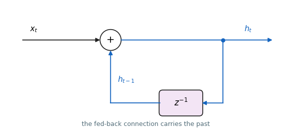
- Store one value, and at every step combine it with the new input: \(h_t = h_{t-1} + x_t\)
- The output at step \(t\) depends on every input so far, through the one stored value
- The delay \(z^{-1}\) is the storage: it hands \(h_t\) to the next step as \(h_{t-1}\)
Cost
- One stored value and one update per step, at any \(t\)
- What is kept is decided by the update rule: a sum keeps the total and loses the individual inputs
Running Statistics Are Memories Kept by Simple Update Rules
Two familiar update rules
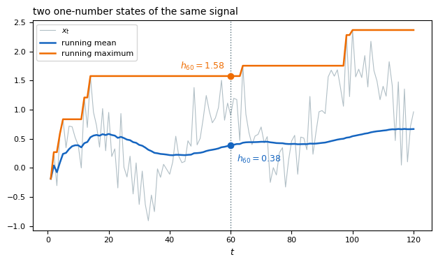
- Running mean: \(h_t = h_{t-1} + (x_t - h_{t-1})/t\), kept with the count \(t\), exact for one statistic of the whole past
- Running maximum: \(h_t = \max(h_{t-1}, x_t)\)
- Each keeps one number computed from every element so far and nothing else
Same loop, different rule
- Both are the accumulator’s loop with a different combination of \(h_{t-1}\) and \(x_t\)
- The rule determines what survives: the mean forgets order and keeps the average, the maximum keeps one extreme value
Recurrent Units Are Feedback Systems
Parts
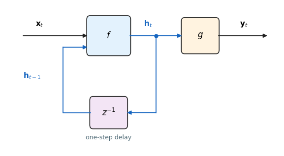
- Input branch: \(\mathbf{x}_t\) enters the block
- State branch: \(\mathbf{h}_{t-1}\) enters through a one-step delay, \(z^{-1}\)
- The block: \(f\), the same at every step
- Readout: \(\mathbf{y}_t = g(\mathbf{h}_t)\), taken off the state
Feedback system
- The delay and the loop make it a discrete-time dynamical system
- Its behavior over many steps is a property of the loop: settling, oscillating, or growing
- Poles, impulse response, stability: the tools for feedback systems apply to this loop unchanged
State Must Forget Most of What It Reads
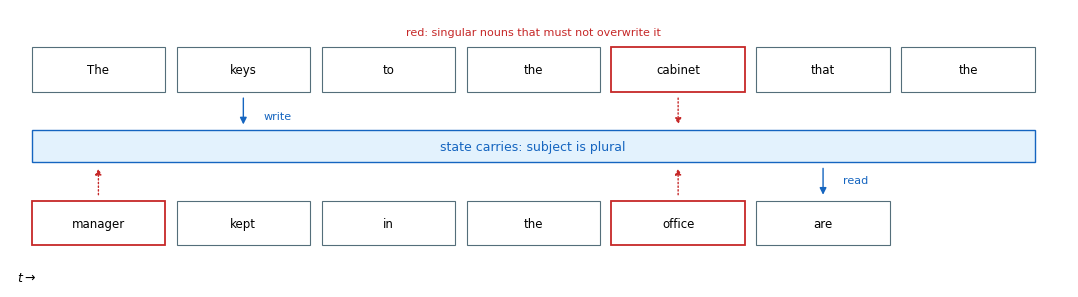
Forgetting is forced
- \(H\) numbers hold \(t\) elements of \(d\) numbers each: once \(t \cdot d > H\), most of the input is discarded
- Every update overwrites part of the state, so keeping one thing means letting another go
Forgetting is chosen at every step
- \(f\) determines what to keep and what to drop when each element arrives, with no access to what comes next
- A useful state forgets the right things: the singular nouns, not the plural subject
Two tasks
- Agreement: hold “plural” from “keys” for eleven tokens, and let three singular nouns pass without overwriting it
- Echo: hold the impulse for 200 steps, then release it
Two questions
- Whether a fixed \(f\) can hold a value for 200 steps at all: the dynamics of the loop
- Whether gradient descent can find such an \(f\): training through the loop
Training Through the Loop Requires Opening It
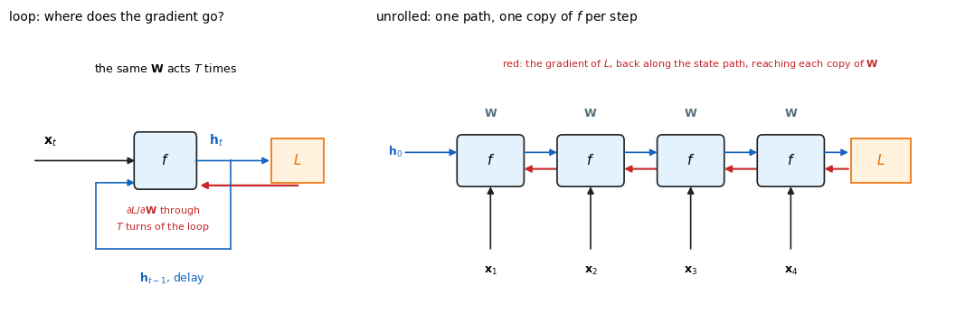
What training needs
- A loss on the output, \(L(\mathbf{y}_T)\) or \(\sum_t L_t(\mathbf{y}_t)\)
- Its gradient with respect to the weights inside \(f\), for gradient descent
- Those weights act at every step, so \(L\) depends on them through every pass around the loop
Why the loop is opened
- In the loop drawing the weights are used once per turn and the turns are not separated: there is no path to draw the gradient along
- Unrolled, every use of the weights is its own copy, the loss sits at the end, and the gradient runs back one copy at a time
- The length of that path is \(T\)
- Same \(f\) and the same weights in every copy: one model, one parameter set, drawn along \(t\)
Unrolled Network Is \(T\) Layers Deep
Depth set by the data
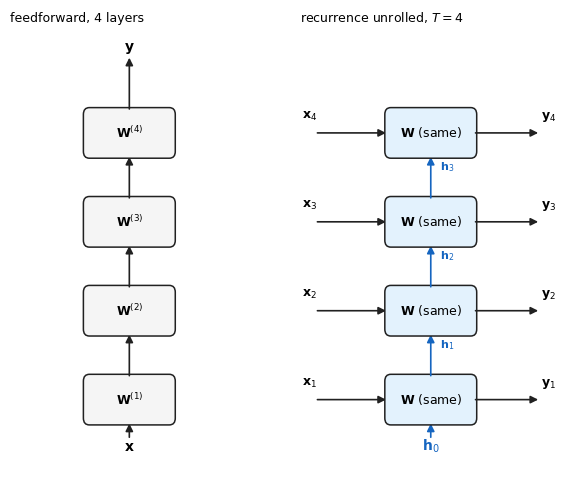
- \(\mathbf{y}_T\) depends on \(\mathbf{x}_1\) through \(T\) applications of \(f\)
- A sentence of 40 tokens is a 40-layer network, a clip of 1000 frames is 1000 layers
Compared with a feedforward network
- Feedforward: \(L\) layers, \(L\) weight matrices, one input at the bottom
- Unrolled recurrence: \(T\) layers, one weight matrix, an input at every layer, an output at every layer
Training
- Training is backpropagation through \(T\) layers of the same weights
- The gradient passes through \(T\) Jacobians, as in any network \(T\) layers deep
- Depth is not a hyperparameter here: the longest example sets it
First-Order Recursion Is a One-Pole Filter
Recursion
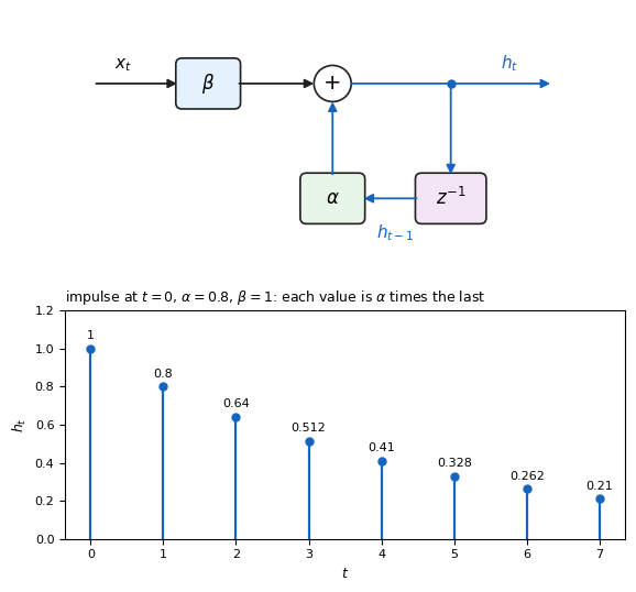
\[h_t = \alpha\, h_{t-1} + \beta\, x_t\]
- One number of state, two coefficients
- \(\beta\): how much of the new input enters
- \(\alpha\): how much of the state survives one step
Impulse response
- Input \(x_0 = 1\), then zero: \(h_t = \beta\,\alpha^t\)
- Every later step multiplies by \(\alpha\) once more
Transfer function
\[H(z) = \frac{\beta}{1 - \alpha z^{-1}}\]
- One pole, at \(z = \alpha\)
- The recurrent unit with \(f\) linear and \(H = 1\)
Pole Location Sets Stability and Memory Length
Three regimes
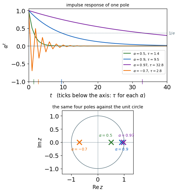
- \(|\alpha| < 1\): every input decays as \(\alpha^t\)
- \(|\alpha| = 1\): an input persists at full strength
- \(|\alpha| > 1\): an input grows without bound
- \(\alpha < 0\): the sign alternates each step, magnitudes unchanged
Memory horizon
- \(\tau = -1/\ln \alpha \approx 1/(1 - \alpha)\): the step at which \(\alpha^t = 1/e\)
- \(\alpha = 0.9\): \(\tau = 9.5\) steps
- \(\alpha = 0.99\): \(\tau = 99.5\) steps
- \(\alpha = 0.999\): \(\tau = 1000\) steps
DC gain
- \(H(1) = \beta / (1 - \alpha)\): the steady output for a constant input of 1
- A longer memory and a larger steady-state gain come from the same \(\alpha\)
Matrix Recursions Have One Pole per Eigenvalue
\[\mathbf{h}_t = \mathbf{A}\mathbf{h}_{t-1} + \mathbf{B}\mathbf{x}_t, \qquad \mathbf{h}_t \in \mathbb{R}^H,\ \mathbf{A} \in \mathbb{R}^{H \times H},\ \mathbf{B} \in \mathbb{R}^{H \times d}\]
Closed form
\[\mathbf{h}_t = \mathbf{A}^t \mathbf{h}_0 + \sum_{i=0}^{t-1} \mathbf{A}^i \mathbf{B}\mathbf{x}_{t-i}\]
- Each input enters through \(\mathbf{B}\), then is multiplied by \(\mathbf{A}\) once per step
Modes
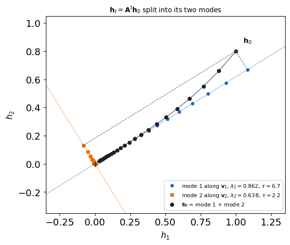
- \(\mathbf{A} = \mathbf{V}\boldsymbol{\Lambda}\mathbf{V}^{-1}\), so \(\mathbf{A}^t = \mathbf{V}\boldsymbol{\Lambda}^t\mathbf{V}^{-1}\)
- In eigen-coordinates \(\tilde{\mathbf{h}} = \mathbf{V}^{-1}\mathbf{h}\), each component evolves alone: \(\tilde{h}_{i,t} = \lambda_i^t\, \tilde{h}_{i,0}\)
- \(H\) poles, one per eigenvalue, each with its own horizon \(-1/\ln|\lambda_i|\)
Spectral radius
- \(\rho(\mathbf{A}) = \max_i |\lambda_i|\), the slowest mode
- \(\rho < 1\): every mode decays. \(\rho = 1\): one mode persists. \(\rho > 1\): one mode grows
- Memory of the whole state: \(\tau \approx -1/\ln\rho\), set by the slowest eigenvalue
Complex Eigenvalues Oscillate Inside the Same Envelope
Complex pair
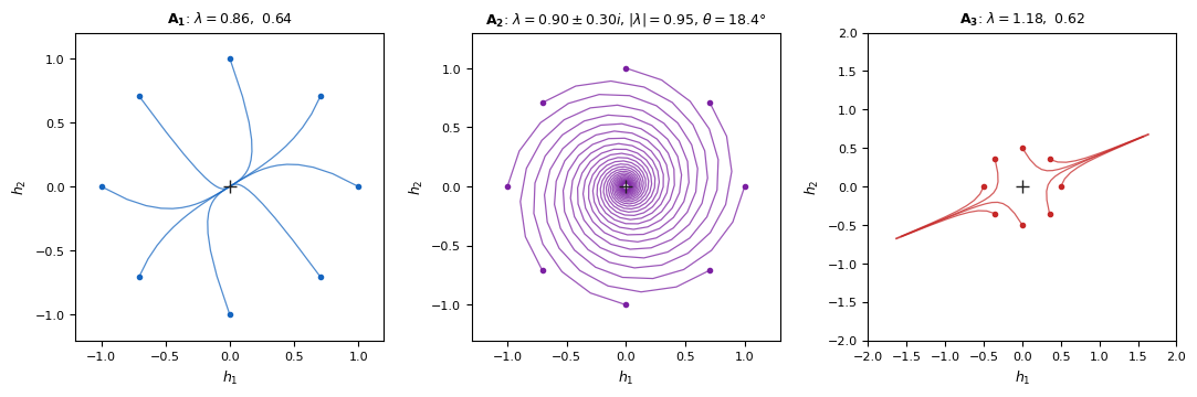
- A real \(\mathbf{A}\) can have \(\lambda = r e^{\pm i\theta}\)
- \(\lambda^t = r^t e^{\pm i t\theta}\): envelope \(r^t\), rotation by \(\theta\) per step
- Period \(2\pi/\theta\) steps, horizon \(-1/\ln r\), set independently
Three \(2 \times 2\) cases
- \(\mathbf{A}_1 = \begin{bmatrix} 0.8 & 0.1 \\ 0.1 & 0.7 \end{bmatrix}\): two real poles inside, decay along two axes
- \(\mathbf{A}_2 = \begin{bmatrix} 0.9 & 0.3 \\ -0.3 & 0.9 \end{bmatrix}\): \(r = 0.95\), \(\theta = 18.4°\), a spiral with period \(19.5\) steps
- \(\mathbf{A}_3 = \begin{bmatrix} 1.1 & 0.2 \\ 0.2 & 0.7 \end{bmatrix}\): one pole outside, decay along one axis and growth along the other
Feedback Trades Stability for Unbounded Reach
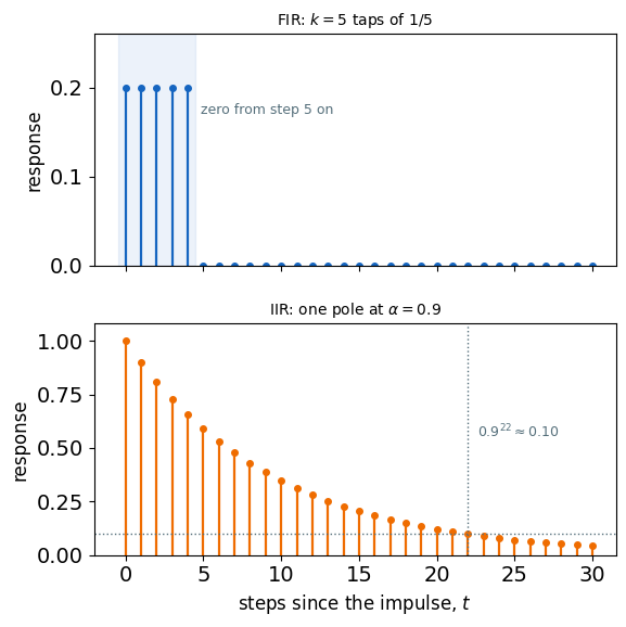
FIR: a window with fixed taps
\[y_t = \sum_{j=0}^{k-1} w_j\, x_{t-j}\]
IIR: feedback through a state
\[h_t = \alpha\, h_{t-1} + \beta\, x_t\]
| FIR (window) | IIR (feedback) | |
|---|---|---|
| Reach | exactly \(k\) steps | unbounded, decaying as \(\alpha^t\) |
| Cost per step | \(k\) multiplications | one for the state, \(H^2\) for a vector state |
| Stability | any taps | $ |
| Sequence model | convolution over time | recurrent unit |
- Reach beyond the window is available only through feedback, and feedback is the only case with a stability condition
Adaptation Is Gradient Descent on the Error Power
Setup
- Target output \(d_t\), filter output \(y_t\), error \(e_t = d_t - y_t\)
- Cost \(J = \mathbb{E}[e_t^2]\), coefficients moved by gradient steps on \(J\)
LMS for FIR taps
\[\mathbf{w}_{t+1} = \mathbf{w}_t + \mu\, e_t\, \mathbf{x}_t\]
- One gradient step per sample, on the instantaneous squared error
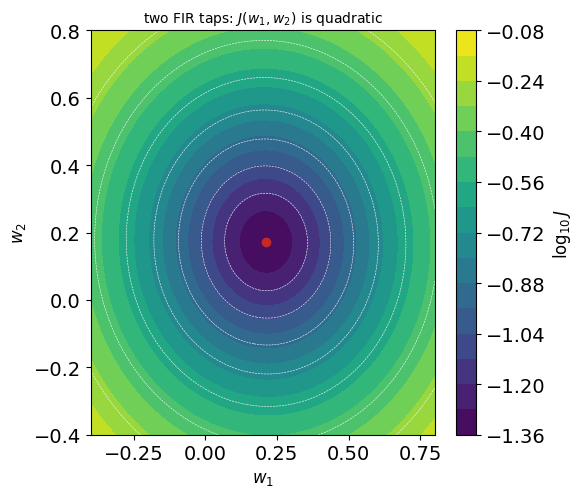
- \(J(\mathbf{w})\) is quadratic in the taps: one minimum, no others
- Converges in the mean for \(\mu < 2/\lambda_{\max}(\mathbf{R}_{xx})\), with \(\mathbf{R}_{xx}\) the input autocorrelation matrix
Same procedure as training a network
- A cost, a gradient, a step size, a stability condition on the step size
- The difference is the shape of \(J\): quadratic here, not in general
Adapting a Feedback Coefficient Sends Gradient Through the Loop
Same setup, one pole to adapt
- \(y_t = \alpha\, y_{t-1} + \beta\, x_t\), cost \(J(\alpha, \beta) = \mathbb{E}[e_t^2]\)
Gradient as a recursion
\[\frac{\partial y_t}{\partial \alpha} = y_{t-1} + \alpha\, \frac{\partial y_{t-1}}{\partial \alpha}\]
- \(y_t\) depends on \(\alpha\) through every earlier output
- The derivative has its own state, updated through the same loop as the signal
- Its magnitude follows the same \(\alpha^t\) as the impulse response
Two consequences
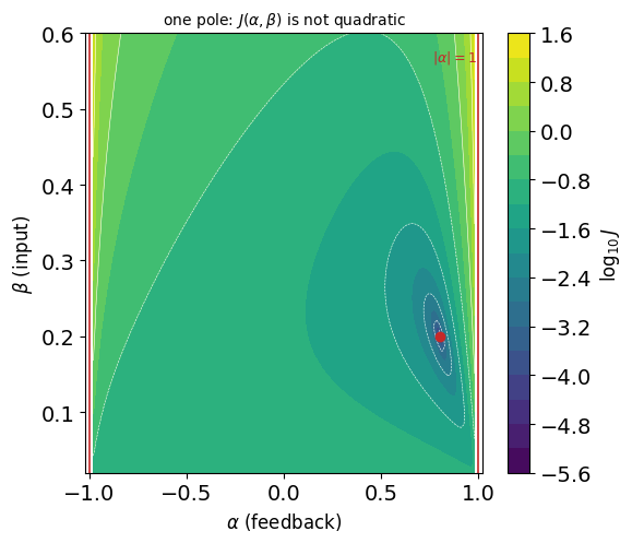
- \(J(\alpha, \beta)\) is not quadratic: a curved valley, steep walls
- Every step must keep \(|\alpha| < 1\). One step across the unit circle and the filter and its gradient both diverge
Carried forward
- A recurrent network trained by gradient has both properties, with \(\alpha\) replaced by a matrix and a nonlinearity in the loop
Linear Filters Cannot Threshold or Latch
Superposition
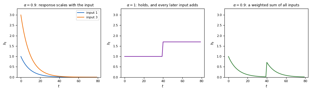
- Response to a sum of inputs is the sum of the responses
- Response to \(3x\) is \(3\) times the response to \(x\)
- The state is always \(\sum_k \alpha^k \beta\, x_{t-k}\): fixed weights, every input counted
What no choice of \(\alpha\), \(\beta\) gives
- A threshold: respond to inputs above a level and not below
- A gate: let one input in and keep another out
- A latch: hold a value against decay, then release it on a signal
- Each needs the coefficients themselves to depend on the signal, or a nonlinearity inside the loop
The recurrent unit’s \(f\) is nonlinear for this reason.
Each Weight Matrix Has One Role
| Object | Shape | Role |
|---|---|---|
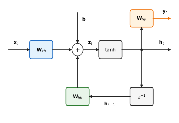
| \(\mathbf{x}_t\) | \(\mathbb{R}^d\) | input at step \(t\) |
| \(\mathbf{h}_t\) | \(\mathbb{R}^H\) | state, the only carrier of the past |
| \(\mathbf{y}_t\) | \(\mathbb{R}^K\) | output at step \(t\) |
| \(\mathbf{W}_{xh}\) | \(\mathbb{R}^{H \times d}\) | projects the input into the state space |
| \(\mathbf{W}_{hh}\) | \(\mathbb{R}^{H \times H}\) | feedback: mixes the state with itself, once per step |
| \(\mathbf{b}\) | \(\mathbb{R}^H\) | sets where on \(\tanh\) the unit operates |
| \(\mathbf{W}_{hy}\) | \(\mathbb{R}^{K \times H}\) | reads the state out, one row per output |
Two of the three are outside the loop
- \(\mathbf{W}_{xh}\) acts on each input once, \(\mathbf{W}_{hy}\) on each state once
- \(\mathbf{W}_{hh}\) acts on the same signal at every step: the only matrix whose repeated application shapes the memory
Time Is the One Axis Hardware Cannot Parallelize
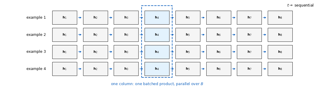
Cost of one step
- \(\mathbf{W}_{hh}\mathbf{h}_{t-1}\): \(H^2\) multiply-adds. \(\mathbf{W}_{xh}\mathbf{x}_t\): \(Hd\). Readout: \(KH\)
- The same at every step, so a sequence costs \(T\) times one step
Parallel axes
- Across the batch: one matrix product per step for all \(B\) examples
- Across outputs: the readout applied to all \(T\) states after the loop
- Not across time: step \(t\) waits for step \(t - 1\)
- Throughput is set by \(B\) and \(H\). A longer \(T\) adds steps in sequence
Backward Pass Needs Every State the Forward Pass Produced
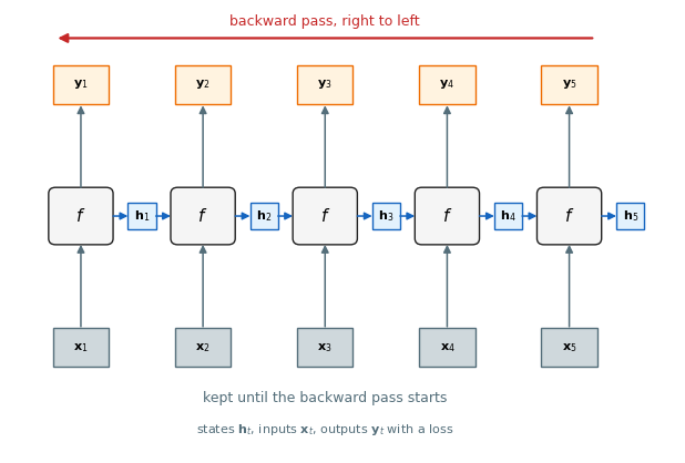
What the backward pass reads
- \(\mathbf{h}_t\) at every step: the gradient through \(\tanh\) at step \(t\) is \(1 - \mathbf{h}_t^2\)
- \(\mathbf{x}_t\) at every step, for the gradient of \(\mathbf{W}_{xh}\)
- \(\mathbf{y}_t\) wherever a loss is attached
Memory, float32, batch \(B\)
| Tensor | Bytes |
|---|---|
| states | \(B \cdot T \cdot H \cdot 4\) |
| inputs | \(B \cdot T \cdot d \cdot 4\) |
| outputs | \(B \cdot T \cdot K \cdot 4\) |
- \(B = 32\), \(T = 100\), the configuration above: \(6.5\) MB of states, \(3.8\) MB of inputs, \(128\) MB of outputs
- Weights, gradients, and Adam’s two moments: \(89\) MB, independent of \(T\)
Growth with \(T\)
- Activation memory grows with \(B \cdot T\) and passes the fixed part before \(T = 100\) at this batch size
- The forward pass cannot free anything: the whole chain is held until the loss is known
One Forward Pass Is a Loop over \(t\)
def rnn_forward(x, h0, W_xh, W_hh, b, W_hy):
    # x: (B, T, d)   h0: (B, H)
    B, T, d = x.shape
    h = h0
    states, outputs = [], []
    for t in range(T):
        z = x[:, t, :] @ W_xh.T + h @ W_hh.T + b   # (B, H)
        h = torch.tanh(z)                          # (B, H)
        y = h @ W_hy.T                             # (B, K)
        states.append(h)
        outputs.append(y)
    return torch.stack(outputs, 1), torch.stack(states, 1)
    # outputs: (B, T, K)   states: (B, T, H)
Line by line
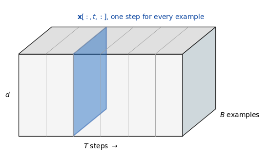
x[:, t, :]: the batch’s step \(t\), one \(B \times d\) slice of the \((B, T, d)\) tensor above. Rows are examples and never interact- Two matrix products and an add: the whole cost of a step
hoverwritten each step: the loop itself needs \(O(BH)\) memorystateskept for the backward pass- Shorter sequences are padded to the longest in the batch and their pad steps masked out of the loss
output Holds Every Step and h_n Holds the Last
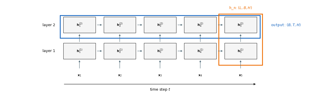
One output for the sequence
- Read
h_n[-1], the top layer’s final state, oroutput[:, -1]: the same tensor - With padding, the final state of each example is at its own length, not at \(T\)
One output per step
- Read
output, all \(T\) states of the top layer, then apply the readout to every step at once - Lower layers’ states are not returned per step. A second
nn.RNNapplied tooutputadds a layer
Stacking Layers Adds Depth at Every Step
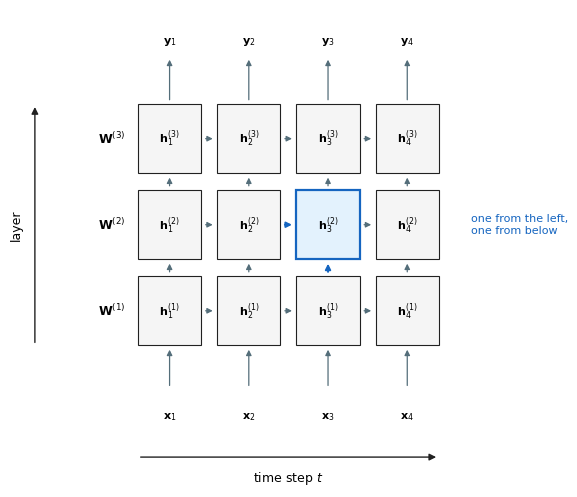
Layer \(l\) takes layer \(l - 1\)’s state as its input
\[\mathbf{h}^{(l)}_t = \tanh\!\left(\mathbf{W}^{(l)}_{hh}\mathbf{h}^{(l)}_{t-1} + \mathbf{W}^{(l)}_{xh}\mathbf{h}^{(l-1)}_t + \mathbf{b}^{(l)}\right), \qquad \mathbf{h}^{(0)}_t = \mathbf{x}_t\]
- Each layer has its own \(\mathbf{W}_{hh}\), \(\mathbf{W}_{xh}\), and state
- Information flows along \(t\) within a layer and up through \(l\) within a step
Cost
- Parameters: \(H^2 + Hd\) for the first layer, \(2H^2\) for each layer above it
- Compute per step: \(L\) times the single-layer recurrence, still sequential in \(t\)
- Memory: \(L\) sets of states kept for training
Depth
- Speech and translation models use two to four layers
- Beyond that, gains are small and the gradient path through \(l\) adds to the path through \(t\)
Bidirectional Layers Read the Sequence in Both Directions
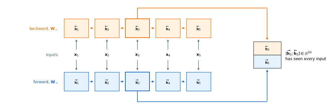
Two units, two directions, one output
- Forward: \(\overrightarrow{\mathbf{h}}_t\) from \(\mathbf{x}_1\) to \(\mathbf{x}_t\). Backward: \(\overleftarrow{\mathbf{h}}_t\) from \(\mathbf{x}_T\) down to \(\mathbf{x}_t\)
- Concatenated per step:
outputis \((B, T, 2H)\),h_nis \((2L, B, H)\) - Twice the parameters and compute of one direction
Requirements
- The whole sequence must exist before the backward pass starts: tagging, offline recognition, an encoder
- Not for prediction as data arrives, and not for generating one element at a time
- A bidirectional layer cannot run online
Backpropagation Through Time Is Backpropagation on the Unrolled Graph
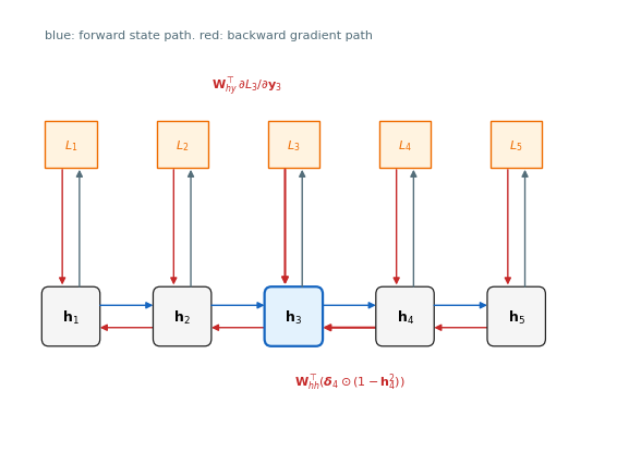
Where the loss sits
- One term per step, \(L = \sum_t L_t\), or one term at the end, \(L = L_T\); a mask \(m_t\) covers both and the padded case
- Gradient enters at each output with a term and nowhere else: an early step is reached only back along the state path
One node, two incoming gradients
\[\boldsymbol{\delta}_t \equiv \frac{\partial L}{\partial \mathbf{h}_t} = \underbrace{\mathbf{W}_{hy}^{\top} \frac{\partial L_t}{\partial \mathbf{y}_t}}_{\text{from this step's output}} + \underbrace{\mathbf{W}_{hh}^{\top}\left(\boldsymbol{\delta}_{t+1} \odot (1 - \mathbf{h}_{t+1}^2)\right)}_{\text{from the next state}}\]
- Start at the end: \(\boldsymbol{\delta}_T\) has the first term only
- Step backward: each \(\boldsymbol{\delta}_t\) needs \(\boldsymbol{\delta}_{t+1}\), so the sweep runs \(T, T-1, \ldots, 1\)
- The second term is the transpose of the forward step: \(\mathbf{h}_{t+1} = \tanh(\mathbf{W}_{hh}\mathbf{h}_t + \ldots)\) forward, \(\mathbf{W}_{hh}^{\top}\) times the \(\tanh\) slope backward
Same recursion as the adaptive one-pole filter
- There: \(\partial y_t / \partial \alpha = y_{t-1} + \alpha\, \partial y_{t-1}/\partial \alpha\), a state passed forward
- Here: a state \(\boldsymbol{\delta}_t\) passed backward, through \(\mathbf{W}_{hh}^{\top}\) instead of \(\alpha\)
Truncation Trains in Windows and Carries the State Across
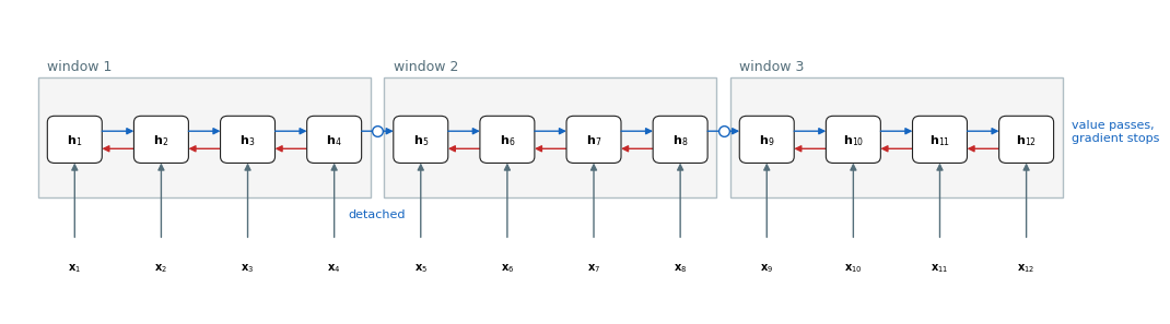
Procedure
- Forward over the whole sequence, in windows of \(k\) steps
- Backward inside each window: gradient of that window’s losses through \(k\) steps of state
- At the window boundary the state is detached:
h = h.detach(), value kept, graph cut
Cost
- Memory: \(k\) states instead of \(T\), so \(T\) can be as long as the data
- Time: the same \(T\) forward and \(T\) backward steps, in pieces
Not trained
- No gradient crosses a boundary: a loss in window 3 cannot adjust how window 1 stored its inputs
- Dependencies longer than \(k\) are never trained, only carried
- \(k = 35\) in the Penn Treebank language models of Zaremba et al. 2014
h = h0
for chunk in sequence.split(k, dim=1):
    h = h.detach()                 # cut the graph here
    out, h = rnn(chunk, h)         # value carried forward
    loss = criterion(out, targets_for(chunk))
    loss.backward(); opt.step(); opt.zero_grad()
Stacked Layers Add One Factor per Layer to Every Gradient Path
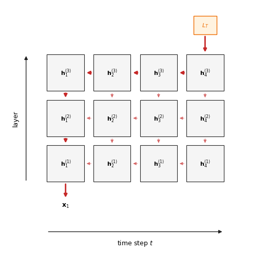
Two kinds of backward step
- Back in time within layer \(l\): \(\mathrm{diag}(1 - \mathbf{h}^{(l)\,2}_t)\,\mathbf{W}^{(l)}_{hh}\), the factor of the single-layer product
- Down from layer \(l\) to \(l - 1\) at one step: \(\mathrm{diag}(1 - \mathbf{h}^{(l)\,2}_t)\,\mathbf{W}^{(l)}_{xh}\), through the weights that read the lower layer’s state
Paths from the last output to the first input
- Every path takes \(T - 1\) steps back and \(L - 1\) steps down: \(T + L - 2\) factors
- The gradient is the sum over all \(\binom{T + L - 2}{L - 1}\) such paths, each a product of that many Jacobians
- One more layer adds one factor to every path, with the same bound \(\le \sigma_{\max}\) as a time step
Consequence
- Depth and time compound: a stack of \(L\) layers has the single layer’s horizon shortened by the extra factors
- Stacks of eight LSTM layers were trained with residual connections between layers, which give the downward step a Jacobian of one (Wu et al. 2016)
Jacobian Product Shrinks Geometrically Unless Every Factor Stays Near One
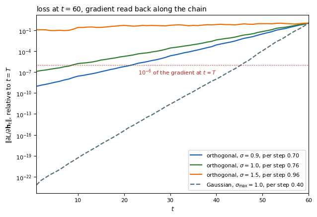
Measured
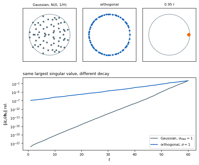
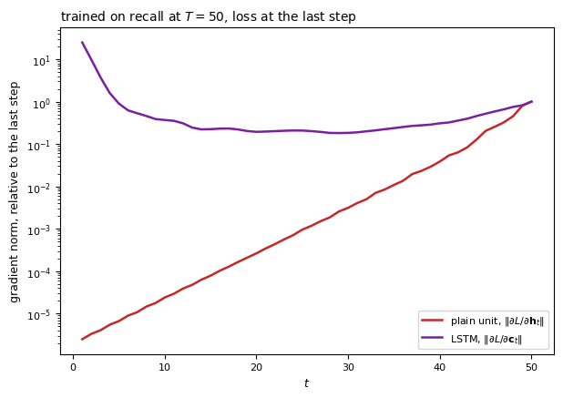
- Each curve is a straight line on the log axis: the decay is geometric, with a per-step factor set by \(\mathbf{W}_{hh}\) and the \(\tanh\) slopes
- Orthogonal at \(\sigma = 1\): about \(0.76\) per step, from the \(\tanh\) slopes alone
- Gaussian at \(\sigma_{\max} = 1\): about \(0.40\) per step, because the state spreads over directions whose singular values are well below 1
Horizon
- Steps until the gradient falls to \(\epsilon\) of its value at \(T\): \(T_\epsilon = \ln \epsilon / \ln \gamma\)
- \(\gamma = 0.76\), \(\epsilon = 10^{-6}\): 50 steps. \(\gamma = 0.40\): 15 steps
- Past the horizon the weights that act at early steps receive no signal from the loss at \(T\)
Recall Falls to Chance Past the Gradient Horizon
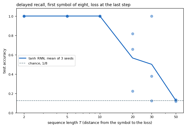
Task
- \(T\) symbols from an alphabet of 8, one-hot
- The first symbol is the target, the other \(T - 1\) are random distractors
- Loss at the last step only: predict the first symbol
- Chance is \(1/8\)
Trained unit
- \(\tanh\) RNN, \(H = 32\), Adam, 1500 steps, three seeds per \(T\)
- Scored on 2000 fresh sequences
Failure
- The state could hold the symbol: 32 numbers for 3 bits
- Vanishing gradient: What fails is training: at \(T = 50\) the loss at the end has no gradient left at step 1, so the weights are never adjusted to write the symbol in a form that survives
Above Scale One the Same Product Explodes
The bound above one
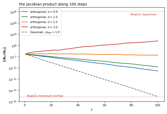
- \(\gamma > 1\): the product grows as \(\gamma^{T-k}\)
- At \(\sigma = 3\): \(10^{12}\) after 100 steps, and the float32 range runs out near \(10^{38}\)
- Between, at \(\sigma = 1.5\): the \(\tanh\) slopes hold the product near one for this input
Symptom in a training run
- A gradient a thousand times its usual size, from one batch
- One parameter update of that size moves the weights to a region where the state saturates or the loss is
nan - The trigger is a state trajectory that passes through a region where several \(\mathbf{J}_t\) are large at once, not the weights alone
Norm Clipping Bounds the Update Without Changing Its Direction
Spikes
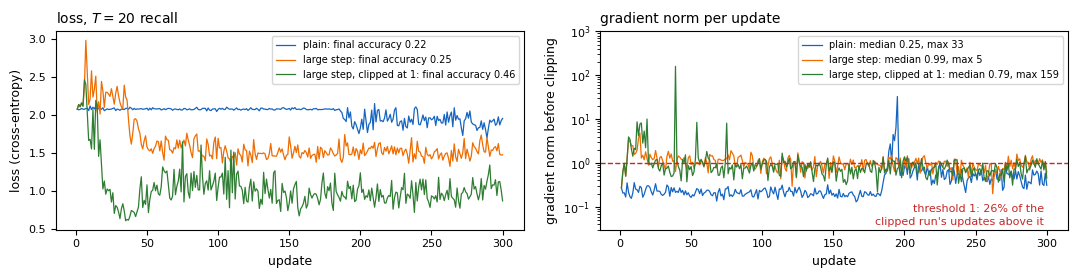
- One batch whose state trajectories pass through a region of large \(\mathbf{J}_t\): the norm jumps two orders of magnitude for one update and returns
- A step small enough for the spike is too small for the other 299 updates, so the bound belongs on the update
Two rules
- Value: each component limited to \([-c, c]\). Changes the direction whenever one component is clipped
- Norm: \(\mathbf{g} \leftarrow \mathbf{g} \cdot \min\!\left(1, c / \|\mathbf{g}\|\right)\). Same direction, length at most \(c\)
torch.nn.utils.clip_grad_norm_(model.parameters(), max_norm=c)
Choosing \(c\)
- From the run: a value the norm crosses on a small fraction of updates, not most of them
- Pascanu et al. 2013 set it from the average norm over many updates
- The clipped large-step run reaches accuracy 0.46 where the unclipped one reaches 0.25
Vanishing untouched
- Nothing for vanishing: a gradient of \(10^{-9}\) is left at \(10^{-9}\)
Orthogonal Initialization Puts Every Singular Value at One
Three starting points for \(\mathbf{W}_{hh}\)
- Gaussian \(\mathcal{N}(0, 1/H)\): eigenvalues fill a disk of radius about 1. Singular values spread from 0 to 2, and most directions of the state are shrunk every step
- Orthogonal: every singular value is 1. A signal in any direction keeps its length through \(\mathbf{W}_{hh}\); only the \(\tanh\) slopes shrink it
- Identity, scaled: \(\mathbf{h}_t \approx 0.95\,\mathbf{h}_{t-1} + \ldots\) at the start, a state that copies itself
First updates only
- The first updates: a Gaussian start at \(\sigma_{\max} = 1\) has a horizon of 15 steps, an orthogonal one of 50, on the profile above
- Nothing after that: training moves \(\mathbf{W}_{hh}\) off the orthogonal set, and the initializer sets nothing about the \(\tanh\) slopes
Layer Normalization Removes Saturation, Not the Decay
Normalize the pre-activation, every step
\[\hat{\mathbf{z}}_t = \frac{\mathbf{z}_t - \mu(\mathbf{z}_t)}{\sigma(\mathbf{z}_t)}, \qquad \mathbf{h}_t = \tanh\!\left(\boldsymbol{\gamma} \odot \hat{\mathbf{z}}_t + \boldsymbol{\beta}\right)\]
- \(\mu\), \(\sigma\) over the \(H\) components of one step of one example: no batch statistics, no running averages
- \(\boldsymbol{\gamma}\), \(\boldsymbol{\beta} \in \mathbb{R}^H\) learned, so the scale is set by training and not by \(\|\mathbf{W}_{hh}\|\)
- Applied inside the loop, to \(\mathbf{z}_t\), not to the output of the module afterwards
Effect
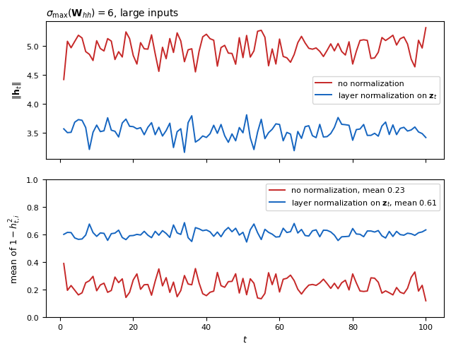
- Saturation: with unit-variance inputs to \(\tanh\) the slopes stay near 0.6 at any weight scale
- Scale drift: \(\|\mathbf{h}_t\|\) no longer depends on \(t\) or on \(\|\mathbf{W}_{hh}\|\)
Unchanged
- The product of \(T\) factors near 0.6 is still \(0.6^T\)
- The horizon moves from 15 steps to 28 at \(\epsilon = 10^{-6}\), and the decay is still geometric
Additive Cell State Passes Gradient Through Unchanged
Additive path
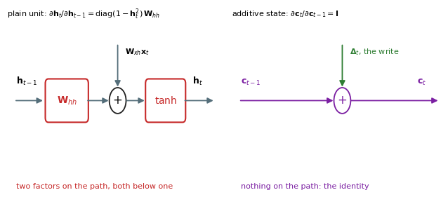
\[\mathbf{c}_t = \mathbf{c}_{t-1} + \boldsymbol{\Delta}_t \qquad \Rightarrow \qquad \frac{\partial \mathbf{c}_t}{\partial \mathbf{c}_{t-1}} = \mathbf{I}\]
- No weight matrix and no \(\tanh\) between \(\mathbf{c}_{t-1}\) and \(\mathbf{c}_t\)
- \(\partial \mathbf{c}_T / \partial \mathbf{c}_k = \mathbf{I}\) for any \(T - k\): the gradient at step \(T\) arrives at step \(k\) at full size
- The write \(\boldsymbol{\Delta}_t\) can still be a nonlinear function of the input and the state
Unconditional sum
- Nothing is ever removed: \(\mathbf{c}_t\) is the sum of every write so far and grows without bound
- Every write is added at full strength, regardless of the current value
- Reading \(\mathbf{c}_t\) out means reading an unbounded quantity
Gates
- Three coefficients in \((0, 1)\), set by the network at every step: how much of \(\mathbf{c}_{t-1}\) to keep, how much of the write to add, how much of the result to read out
Forget Gate Is the Pole of Each Cell Dimension
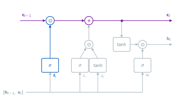
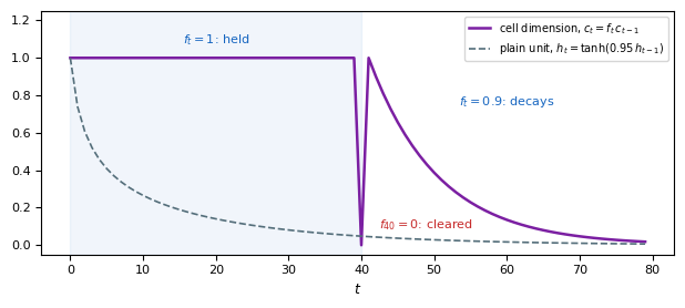
Forget gate on the cell line
\[\mathbf{f}_t = \sigma\!\left(\mathbf{W}_f[\mathbf{h}_{t-1}, \mathbf{x}_t] + \mathbf{b}_f\right), \qquad \mathbf{c}_t = \mathbf{f}_t \odot \mathbf{c}_{t-1} + \ldots\]
\[\frac{\partial \mathbf{c}_t}{\partial \mathbf{c}_{t-1}} = \mathrm{diag}(\mathbf{f}_t)\]
- One coefficient per dimension, in \((0, 1)\): a pole inside the unit circle, placed by the network at every step
- \(f = 1\): that dimension is held exactly. \(f = 0\): cleared. Between: decay at \(f^t\)
- No weight matrix on the path: the Jacobian is the gate values themselves
Three regimes of a gate value
- \(f \to 1\): the signal passes at full strength. \(f \to 0\): cut. Between: a scaling, and the only range where \(\sigma\) has a nonzero slope
- The one-pole filter’s \(\alpha\), set from the signal itself at every step and for every dimension
Initialization
- \(\mathbf{b}_f\) set to 1 or 2 at the start: \(\sigma(1) = 0.73\), \(\sigma(2) = 0.88\)
- The cell starts by retaining, and training lowers the gates of the dimensions that should forget
- A gate that starts near 0 clears the cell at every step, so no long dependency is ever visible to the gradient
Each Write Is an Amount Times a Value
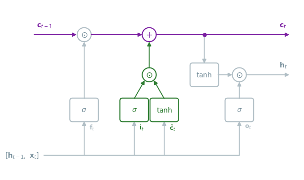
Two parts to a write
\[\mathbf{i}_t = \sigma\!\left(\mathbf{W}_i[\mathbf{h}_{t-1}, \mathbf{x}_t] + \mathbf{b}_i\right), \qquad \tilde{\mathbf{c}}_t = \tanh\!\left(\mathbf{W}_c[\mathbf{h}_{t-1}, \mathbf{x}_t] + \mathbf{b}_c\right)\]
\[\mathbf{c}_t = \mathbf{f}_t \odot \mathbf{c}_{t-1} + \mathbf{i}_t \odot \tilde{\mathbf{c}}_t\]
- \(\tilde{\mathbf{c}}_t \in (-1, 1)^H\): the content, signed, the same form as the plain unit’s update
- \(\mathbf{i}_t \in (0, 1)^H\): how much of it enters, per dimension
- Separating the two lets the network compute a candidate at every step and write it only on inputs that require it
Against the plain unit
- Plain: \(\mathbf{h}_t = \tanh(\ldots)\), the whole state replaced by the update at every step
- Here: the old value survives through \(\mathbf{f}_t\) and the update is added, scaled by \(\mathbf{i}_t\)
- With \(\mathbf{f}_t = 0\) and \(\mathbf{i}_t = 1\) the cell is the plain unit’s update. With \(\mathbf{f}_t = 1\) and \(\mathbf{i}_t = 0\) it is a constant
Output Gate Sets What the Rest of the Network Reads
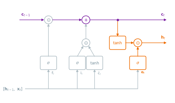
Read path
\[\mathbf{o}_t = \sigma\!\left(\mathbf{W}_o[\mathbf{h}_{t-1}, \mathbf{x}_t] + \mathbf{b}_o\right), \qquad \mathbf{h}_t = \mathbf{o}_t \odot \tanh(\mathbf{c}_t)\]
- \(\mathbf{c}_t\) is unbounded: a dimension held at \(f = 1\) and written to repeatedly grows
- \(\tanh(\mathbf{c}_t)\) bounds the read to \((-1, 1)\) without changing the stored value
- \(\mathbf{o}_t\) selects, per dimension, how much of the bounded read leaves the cell
Two states
- \(\mathbf{c}_t\) stays inside the cell. \(\mathbf{h}_t\) goes to the readout and back into the input of every gate at \(t + 1\)
- A dimension can be held in \(\mathbf{c}_t\) for many steps while \(\mathbf{o}_t\) keeps it out of \(\mathbf{h}_t\) until a later step reads it
LSTM Cell Is One Additive Path and Three Gates
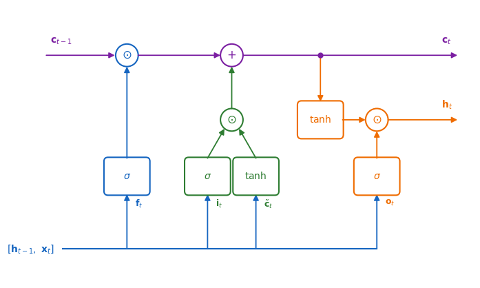
\[\begin{aligned}
\mathbf{f}_t &= \sigma(\mathbf{W}_f[\mathbf{h}_{t-1}, \mathbf{x}_t] + \mathbf{b}_f) & \mathbf{i}_t &= \sigma(\mathbf{W}_i[\mathbf{h}_{t-1}, \mathbf{x}_t] + \mathbf{b}_i) \\
\tilde{\mathbf{c}}_t &= \tanh(\mathbf{W}_c[\mathbf{h}_{t-1}, \mathbf{x}_t] + \mathbf{b}_c) & \mathbf{o}_t &= \sigma(\mathbf{W}_o[\mathbf{h}_{t-1}, \mathbf{x}_t] + \mathbf{b}_o) \\
\mathbf{c}_t &= \mathbf{f}_t \odot \mathbf{c}_{t-1} + \mathbf{i}_t \odot \tilde{\mathbf{c}}_t & \mathbf{h}_t &= \mathbf{o}_t \odot \tanh(\mathbf{c}_t)
\end{aligned}\]
One step, in order
- Four affine maps of the same input \([\mathbf{h}_{t-1}, \mathbf{x}_t]\), one \(\sigma\) or \(\tanh\) each
- Scale the old cell by \(\mathbf{f}_t\), add the scaled candidate
- Bound the new cell with \(\tanh\), scale by \(\mathbf{o}_t\), output as \(\mathbf{h}_t\)
- Four matrices of \(H \times (H + d)\) on one concatenated input, one addition
- Only the addition is on the path from \(\mathbf{c}_{t-1}\) to \(\mathbf{c}_t\)
Gradient Along the Cell Is a Product of Gates
Along the cell line
\[\frac{\partial \mathbf{c}_T}{\partial \mathbf{c}_k} = \prod_{t=k+1}^{T} \mathrm{diag}(\mathbf{f}_t) + (\text{terms through } \mathbf{h}_t)\]
- The first term is an elementwise product of numbers in \((0, 1)\), one per dimension
- No \(\mathbf{W}_{hh}\) and no \(\tanh\) slope in it: the network sets the factors directly, through the gates
- A dimension whose gate stays at \(0.99\) passes \(0.99^{100} = 0.37\) of the gradient across 100 steps, and at \(1.0\) all of it
Other terms
- \(\mathbf{f}_t\), \(\mathbf{i}_t\), \(\tilde{\mathbf{c}}_t\) depend on \(\mathbf{h}_{t-1}\), which depends on \(\mathbf{c}_{t-1}\): a second path, through the gates’ weight matrices
- That path has the plain unit’s structure and decays as before. The cell line carries gradient without it
Measured on the trained units
- Same recall task, \(T = 50\), seed 0: the plain unit at chance, the LSTM at 100%
- Gradient of the final loss read back along \(\mathbf{c}_t\) (LSTM) and \(\mathbf{h}_t\) (plain unit)
Gated Unit Recalls Past the Plain Unit’s Horizon
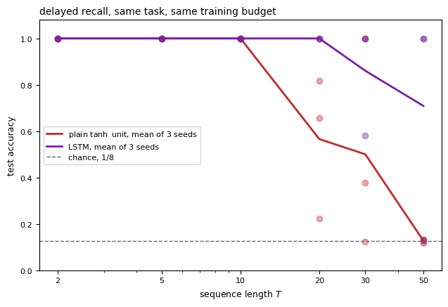
Same task, same budget
- \(H = 32\) for both, Adam at the same rate, 1500 steps, three seeds
- LSTM forget-gate bias set to 2 at the start
Measured
- Plain unit: 100% through \(T = 10\), chance at \(T = 50\) for every seed
- LSTM: 100% through \(T = 20\) for every seed, 100% at \(T = 50\) for two seeds of three
Failed seed
- One LSTM seed sits at chance at \(T = 50\): the additive path makes long recall trainable and does not guarantee that training reaches it
- Whether training reaches the hold-then-read solution depends on the initial weights
GRU Keeps One State and Couples Its Two Gates
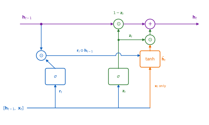
\[\begin{aligned}
\mathbf{z}_t &= \sigma(\mathbf{W}_z[\mathbf{h}_{t-1}, \mathbf{x}_t] + \mathbf{b}_z) & \mathbf{r}_t &= \sigma(\mathbf{W}_r[\mathbf{h}_{t-1}, \mathbf{x}_t] + \mathbf{b}_r) \\
\tilde{\mathbf{h}}_t &= \tanh(\mathbf{W}[\mathbf{r}_t \odot \mathbf{h}_{t-1},\ \mathbf{x}_t] + \mathbf{b}) & \mathbf{h}_t &= (1 - \mathbf{z}_t) \odot \mathbf{h}_{t-1} + \mathbf{z}_t \odot \tilde{\mathbf{h}}_t
\end{aligned}\]
Three changes from the LSTM
- One state: \(\mathbf{h}_t\) is both what is stored and what is read, so no output gate and no \(\tanh\) on the read
- Coupled gates: forget is \(1 - \mathbf{z}_t\) and write is \(\mathbf{z}_t\), so the update is a convex combination and the state stays bounded
- Reset gate: \(\mathbf{r}_t\) scales the old state going into the candidate only, not the old state that is kept
Same additive path
- \(\partial \mathbf{h}_t / \partial \mathbf{h}_{t-1} = \mathrm{diag}(1 - \mathbf{z}_t) + \ldots\): a product of gate values again
- Three affine maps instead of four: \(3H(H + d + 1)\) parameters, three quarters of the LSTM’s cost
- Accuracy within one to two points of the LSTM, in either direction, on the tasks of Chung et al. 2014
Output Count Is Set by the Input
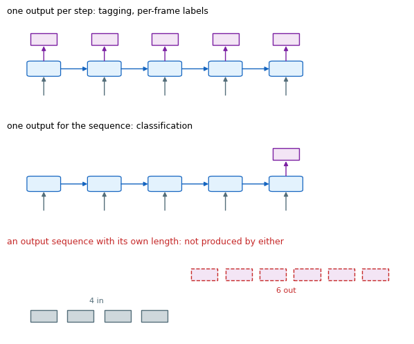
Two readings of one unit
- A readout on every state: one output per input element, \(T\) in, \(T\) out
- A readout on the last state: one output for the whole input, \(T\) in, \(1\) out
Both are set by the input
- The number of outputs is \(T\) or \(1\), and the positions of the outputs are the positions of the input
- Tagging, per-frame recognition, and sentence classification fit these shapes
Tasks that do not
- An output that is itself a sequence, with a length and an order of its own: a sentence produced from a sentence, a sentence produced from an image
Final State Is a Fixed-Size Summary of the Whole Input
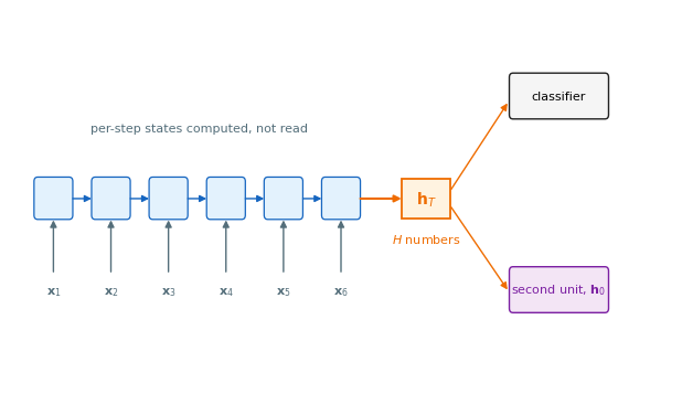
One vector for any length
- Run the unit to the end of the input and keep only \(\mathbf{h}_T \in \mathbb{R}^H\)
- Six steps or six hundred: the same \(H\) numbers
Two consumers
- A classifier: the sequence-classification reading of the previous slide
- Another recurrent unit, as its initial state: the vector becomes the starting memory of a second loop
Trained from where it is read
- Every gradient that shapes \(\mathbf{h}_T\) enters at step \(T\) and reaches step \(t\) through \(T - t\) Jacobians
- What the summary keeps from early inputs is limited by the horizon measured earlier in the training section, and by the gates
Units Fed Their Own Output Produce Sequences of Any Length
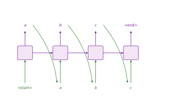
One added connection
- The readout produces a distribution over symbols, one symbol is chosen, and that symbol is the next input
- The unit’s own outputs drive it: no input sequence is needed after the first symbol
Length set by the unit
- The loop stops when it chooses an end symbol
- The number of outputs is no longer the number of inputs
What sets the first state
- With \(\mathbf{h}_0 = \mathbf{0}\) the unit produces sequences from what it learned alone
- With \(\mathbf{h}_0\) from another unit’s final state, what it produces depends on that unit’s input
Two Units Joined Through One State Map a Sequence to a Sequence
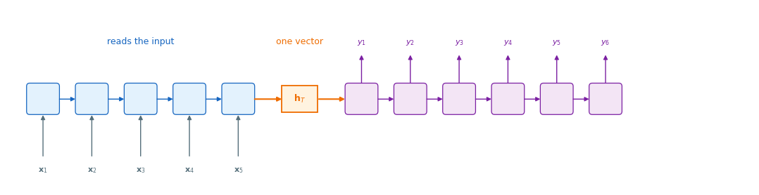
The composition
- First unit: reads the input, keeps only its final state
- Second unit: starts from that state and produces outputs by feeding back its own choices
- Input length and output length are independent, and both are set by the data
What it demands of one vector
- Everything the second unit uses about the input passes through \(\mathbf{h}_T\), \(H\) numbers
- That vector must carry the first input across every later input of the first unit, then across every output of the second
- The gated unit makes that path trainable. Whether \(H\) numbers are enough for a long input is a separate question